Instructions

Buttons for search

• depth-first: Depth-first search, optimizing depth. Distances between landmarks are ignored. The queue is last in first out.
• breadth-first: Breadth-first search, optimizing depth. Distances between landmarks are ignored. The queue is first in first out, so the shallower (lesser depth) is always pulled out first. It is identical to uninformed cost-based if the cost of each path is set to be identically $1$ (i.e. uniform-cost).
• uninformed cost-based: Search optimizing the distance (i.e. the cost). It is uninformed because it does not use any information (i.e. heuristic) on how close the landmark is from the goal. The node in the queue with the lowest distance traversed ($z$) is extracted first.
• heuristic greed-first: Also optimizes the distance. The node in the queue with closest to the goal (least $h$) is extracted first. It uses the A* distance ($a^* = z + h$) to determine if some nodes are non-optimal and should be terminated and not extended.
• A*: Also optimizes the distance. The node in the queue with the least A* distance $a^* = z + h$ is extracted first. It also uses the A* distance to determine if some nodes are non-optimal and should be terminated and not extended.

Buttons for fine adjustments

• Click on a landmark and then "set as start" will assign that point to be the starting point. set as end assigns the end point.
• Click on one landmark after another then click "toggle path" to connect/disconnect the two landmarks.
• If "do not amputate" is selected then a search will extend the detour nodes (orange nodes, see terminology below) even though they will not lead to the optimal path. This is used to illustrate the extra computational burden if the search tree is not amputated efficiently (although there is extra memory cost to identify the detour notes, not visible in this simulation). Note that non-optimal nodes (red nodes, see terminology below) are still not expanded even when "do not amputate" is clicked because non-optimal nodes can usually be identified without much additional memory cost.
• "simplify tree" will remove all detour nodes (orange) and non-optimal nodes (red, see terminology below) making the tree easier to study.
• "show full tree" undo the tree simplification and restore all nodes. The full tree is useful in seeing what decisions are made by the program to truncate the nodes.

Draggables and clickables

• Landmarks and tree nodes can be moved by dragging.
• Clicking on a node (middle view) reveals the corresponding path in the map (top view). This is disabled during path finding.

Sliders

• fast forward / slow motion: controls the speed of the simulation.
• maximum connection length: When it is at $100\%$ then all map connections are possible. For example, if set to $70\%$, then connections in the map cannot be longer than $70\%$ the width of the map view.
• likihood to disconnect: The larger the value, the less connections are formed among the landmarks.
• number of landmarks: Self explanatory.

Terminology

• Map: Collection of landmarks and connections (top view).
• Landmark: A location in the map (top view). Note that each landmark could appear in multiple nodes in the tree (middle view).
• Tree: The goal tree (middle view). It represents the results of the search.
• Root: The first node in the tree.
• Node: A node in the tree (middle view). Each node represents a path from the root. Clicking on a node reveals the corresponding path in the map.
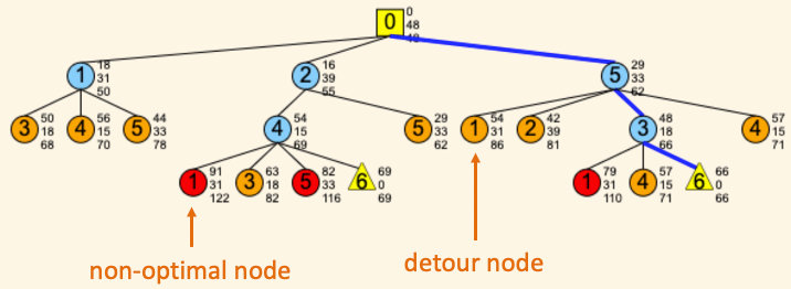
• Detour node: If there is a better path to get to the landmark in the node, then the node is a detour (i.e. longer than is necessary). Detour nodes are painted orange. Detour nodes are always identified by the actual path that has already been traversed. Identifying detour nodes will make the search much more efficient but usually comes with memory cost since previous distances have to be stored.
• Non-optimal node: If there is a better path to get to the goal from the node, then the node is non-optimal. Non-optimal nodes are painted red. Non-optimal nodes can be identified by making use of heuristic distance (if available) and the actual path that has already been traversed. Identifying non-optimal node is usually not as memory intensive as detour nodes, because only the length of the optimal path and the distance of the current path are needed, which are two pieces of information the search needs to keep track of anyway.
• Deadend node: If a node cannot be extended further because the landmark it contains is in a dead-end, then it is a deadend node. Such node are not painted differently than a regular node.
• Goal node: The node contains the goal landmark. There could be multiple goal nodes in a tree because there are more than one way to arrive there. A goal node is drawn as a yellow triangle.
• Active node: The search examines one node at a time. The active node is the one just extracted from the queue. Active node is painted in dodger blue.
• Queue: A list of nodes to be examined. The order in which a node is extracted from the queue is one key in differentiating the search algorithms.
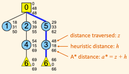
• Distance traversed, $z$: The actual distance of the path leading to the current node. We use the letter $z$ because the path is usually zig-zag like.
• Heuristic distance, $h$: An underestimation (i.e. admissible heuristic) of the distance to the goal. In this simulation we use the straight line distance (i.e. airline distance) as the heuristic distance.
• A* distance, $a^*$: $a^* = z+h$, i.e. A* distance is the sum of the distance traversed and the heuristic distance.

Theory

The key idea

All algorithms differ in two aspects:

1. How the non-optimal nodes and the detour nodes are identified.
2. The order in which the active node is extracted from the queue.

By changing these two aspects, we can generate all the algorithms that are commonly used.

Searching for a path is equivalent to building the goal tree from the root. The key question is where to stop extending the tree. With some thinking, one can see that a node terminates a branch in the goal tree for one of the following reasons (and no other possiblities):

1. Goal node: The node contains the goal. A goal node is a yellow triangle in the goal tree.
2. Deadend node: The node represent a deadend on the map. Such a node is drawn as a regular node.
3. Non-optimal node: There is a better path to get to the goal from this node. Such a node is painted red.
4. Detour node: There is a better path to get to the same landmark contained in the node. Such a node is painted orange. Choosing "do not amputate" will extend these nodes, illustrating the inefficiency if they are kept.

Comparison of the algorithms in the simulation

Algorithm	Queue	Non-optimal node (red)	Detour node (orange)
Depth-first (depth optimizing)	Last in first out (i.e. go as deep as possible each time)	Depth $\geq$ the optimal depth found so far	If landmark in node appears in another node of lesser depth
Breadth-first (depth optimizing)	First in first out (i.e. go layer by layer, shallow to deep)	Depth $\geq$ the optimal depth found so far	If landmark in node appears in another node of lesser depth. Equivalent to checking if another node with the same landmark has already appeared in the tree.
Uninformed cost-based	Minimum $z$ first out (least distance traversed from root)	$z$ to goal is longer than the optimal $z$ found so far	$z$ to landmark in node is longer than the optimal $z$ to the same landmark found so far
Heuristic greed-first	Minimum $h$ first out (closest to goal)	$a^*$ to goal is longer than the optimal $z$ found so far	$z$ to landmark in node is longer than the optimal $z$ to the same landmark found so far
A*	Minimum $a^* = z + h$ first out (lowest estimate of root to goal distance)	$a^*$ to goal is longer than the optimal $z$ found so far	$z$ to landmark in node is longer than the optimal $z$ to the same landmark found so far

Difference of my version with the most common implementations

In heuristic greed-first and A*, the detour nodes are usually identified by keeping a list of already extended landmarks. When the tree comes across a node with a landmark that has already been extended, then the node truncates that branch. However, this only gives the optimal path in A* if the heuristic distance $h$ is both admissible and consistent. While the straight line distance in the map satisfies these requirements, the heuristic greed-first search still could give the non-optimal paths. To avoid such pathological cases, the above criterion in the table is used instead. It has higher memory cost, but ensures the optimal paths in all cases.

Since I am a theoritical physicist, some changes are made in the algorithms to make them more "elegant" (in my view anyway) so all search algorithms can be ran on the same basic codes with minor adjustments, but at a cost that the searches are not performed in the absolutely most efficent way. For example, a large number of nodes could have been excluded from joining the queue to begin with by some pre-filtering, but this is not done for padagogical reason so we can see how all nodes are examined and truncated.

About the simulation

The main concepts behind the simulation is based on the excellent lectures by the late Patrick Winston at MIT (see lecture 4 and lecture 5). The complete course can be found here. Also a big thank to my student A. J. Straight, whose own excellent work on the topic also inspired me to finally sit down and put my thoughts on path finding and how it should be visualized into this simulation.