Area of one turn:
$$
A = \pi r^2 = \pi ([[return ~r~]] \times 10^{-3})^2 = [[return sf_latex(namespace_inductance.A)]] m^2
$$
Inductance:
$$
\begin{eqnarray}
L &=& \mu_0 N^2 A / l \\
&=& (4\pi \times 10^{-7} H/m) ([[return ~N~]]^2) ([[return (namespace_inductance.A * 1e6).toFixed(1)]] \times 10^{-6} m^2) / ([[return ~l~]] \times 10^{-3} m) \\
&=& [[return sf_latex(namespace_inductance.L, 5)]] H \\
&=& [[return sf_latex(namespace_inductance.L * 1e3)]] mH \\
\end{eqnarray}
$$
You can also use the equation $L = \mu_0 n^2 A l$ to get the same answer.
Magnetic field:
$$
\begin{eqnarray}
B &=& \mu_0 n I \\
&=& (4\pi \times 10^{-7} H/m) ([[return sf_latex(namespace_inductance.n)]] m^{-1}) (~i~ A) \\
&=& [[return sf_latex(namespace_inductance.field)]] T
\end{eqnarray}
$$
Flux of one turn:
$$
\begin{eqnarray}
\Phi_1 &=& BA \\
&=& ([[return sf_latex(namespace_inductance.field)]] T) ([[return sf_latex(namespace_inductance.A)]] m^2) \\
&=& [[return sf_latex(namespace_inductance.flux_one_turn)]] Wb
\end{eqnarray}
$$
The ratio $\frac{\Phi_N}{I}$ should just be the inductance (by definition):
$$
\begin{eqnarray}
\frac{\Phi_N}{I} &=& \frac{[[return sf_latex(namespace_inductance.flux_total)]] Wb}{~i~ A} \\
&=& [[return sf_latex(namespace_inductance.L)]] H = L
\end{eqnarray}
$$
The values of two of the variables ($L$, $\Phi_B$, $I$) below has
been given to you. Use that information to calculate the remaining unknowns, including the energy of the inductor $U_B$.
if (int_count_times_randomized == 0){
return 3;
} else {
return random_min_max_precision(1, 10, 0); //defined in setup_exercise_all.js.
}
if (int_count_times_randomized == 0){
return 10;
} else {
return random_min_max_precision(1, 10, 0); //defined in setup_exercise_all.js.
}
if (int_count_times_randomized == 0){
return 0;
} else {
return random_min_max_precision(0, 2, 0); //defined in setup_exercise_all.js.
}
Hint:
Use $L = \frac{\Phi_B}{I}$ to solve for the unknown.
Energy can be found using one of the equations: $U_B = \frac{1}{2}L I^2 = \frac{1}{2}\Phi_B I = \frac{\Phi_B^2}{2L}$.
Solution
From $L = \frac{\Phi_B}{I}$ we get the values for $L$, $\Phi_B$, $I$.
Any of the equations from $U_B = \frac{1}{2}L I^2 = \frac{1}{2}\Phi_B I = \frac{\Phi_B^2}{2L}$ will give the right answer.
For example:
$$
U_B = \frac{1}{2}\Phi_B I = \frac{1}{2}([[return ~~Phi]]) ([[return ~~I]]) = [[return (0.5* ~~Phi * ~~I).toFixed(2)]] J.
$$
$L = $
return (~~Phi / ~~I).toFixed(2);
10%
Unit:
return "H";
not_number
$\Phi_B=$
return ( ~~Phi).toFixed(2);
0.1
Unit:
return "Wb";
not_number
$I=$
return (~~I).toFixed(2);
0.1
Unit:
return "A";
not_number
$U_B=$
return (0.5* ~~Phi * ~~I).toFixed(2);
10%
Unit:
return "J";
not_number
current || inductance
Exercise - Energy density of an inductor
if (int_count_times_randomized == 0){
return 3000;
} else {
return random_min_max_precision(1000, 9000, -3); //defined in setup_exercise_all.js
}
if (int_count_times_randomized == 0){
return 20;
} else {
return random_min_max_precision(10, 30, 0); //defined in setup_exercise_all.js
}
if (int_count_times_randomized == 0){
return 5;
} else {
return random_min_max_precision(2, 10, 1); //defined in setup_exercise_all.js
}
if (int_count_times_randomized == 0){
return 4;
} else {
return random_min_max_precision(1, 10, 0); //defined in setup_exercise_all.js
}
return (true);
A solenoid has the following specifications:
$N = ~N~$: total number of turns.
$l = ~l~ mm$: length of the solenoid.
$r = ~r~ mm$: radius of the cross-section of the solenoid.
$I = ~i~ A$: current flowing through the solenoid.
Find:
The turns density (i.e. turns per unit length, $n$).
The inductance.
The magnetic field inside.
The total energy.
The energy density.
Very big or very small numbers can be entered as "1.234e-6" (for $ 1.234\times 10^{-6}$).
$\mu_0 \approx 4\pi \times 10^{-7} H/m$
Area of one turn:
$$
A = \pi r^2 = \pi ([[return ~r~]] \times 10^{-3})^2 = [[return sf_latex(namespace_inductance.A)]] m^2
$$
Inductance:
$$
\begin{eqnarray}
L &=& \mu_0 N^2 A / l \\
&=& (4\pi \times 10^{-7} H/m) ([[return ~N~]]^2) ([[return (namespace_inductance.A * 1e6).toFixed(1)]] \times 10^{-6} m^2) / ([[return ~l~]] \times 10^{-3} m) \\
&=& [[return sf_latex(namespace_inductance.L, 5)]] H \\
&=& [[return sf_latex(namespace_inductance.L * 1e3)]] mH \\
\end{eqnarray}
$$
You can also use the equation $L = \mu_0 n^2 A l$ to get the same answer.
Magnetic field:
$$
\begin{eqnarray}
B &=& \mu_0 n I \\
&=& (4\pi \times 10^{-7} H/m) ([[return sf_latex(namespace_inductance.n)]] m^{-1}) (~i~ A) \\
&=& [[return sf_latex(namespace_inductance.field)]] T
\end{eqnarray}
$$
if (int_count_times_randomized == 0){
return 10;
} else {
return random_min_max_precision(1, 20, 0); //defined in setup_exercise_all.js
}
if (int_count_times_randomized == 0){
return 1;
} else {
return random_min_max_precision(0, 10, 0); //defined in setup_exercise_all.js
}
if (int_count_times_randomized == 0){
return 9;
} else {
return random_min_max_precision(0, 10, 0); //defined in setup_exercise_all.js
}
if (int_count_times_randomized == 0){
return 2;
} else {
return random_min_max_precision(1, 50, 0); //defined in setup_exercise_all.js
}
return (true);
An inductor with a changing current.
The figure shows a current passing through an inductor with inductance $~inductance~ mH$. Initially the current is $I_1 = ~i_1~ A$. After $~t~ ms$ ("milliseconds"), the current is $I_2 = ~i_2~ A$. Find the self-induced emf (include the sign) and its direction.
Change in current:
$$
\begin{eqnarray}
\Delta I &=& I_2 - I_1 \\
&=& ~i_2~ A - ~i_1~ A \\
&=& [[return sf_latex(namespace_inductance.i_delta)]] A
\end{eqnarray}
$$
$\mathcal{E}_L [[return (namespace_inductance.emf>0)? "\\gt":"\\lt"]] 0$ means the emf is in the [[return (namespace_inductance.emf>0)? "same":"opposite"]] direction to the current.
Since $I_1 = I_2 = ~i_1~ A$, there is no change in the current. In this case no emf is induced, so $\mathcal{E}_L = 0V$.
$\mathcal{E}_L= $
return sf_math(namespace_inductance.emf)
5%
Direction of emf =
if (~i_1~ == ~i_2~){
return "zero";
} else if (namespace_inductance.emf > 0){
return "down";
} else {
return "up";
}
not_number
(type "up", "down", or "zero" for no current)
Select unit for $\mathcal{E}_L$:
$V$
$V/m$
$A/s$
$H$
0
current || inductance || circuit
Exercise - "Charging" an inductor
if (int_count_times_randomized == 0){
return 12;
} else {
return random_min_max_precision(3, 20, 0); //defined in setup_exercise_all.js
}
if (int_count_times_randomized == 0){
return 4;
} else {
return random_min_max_precision(3, 5, 1); //defined in setup_exercise_all.js
}
if (int_count_times_randomized == 0){
return 24;
} else {
return random_min_max_precision(10, 30, 0); //defined in setup_exercise_all.js
}
return 1;
return (true);
"Charging" in an $RL$ circuit.
A inductor with $L = ~l~ H$ is "charged" by a battery with emf $\mathcal{E} = ~v_0~ V$, through a resistor $R = ~r~ \Omega$.
Calculate the following:
Time constant $\tau$.
Maximum current on the inductor $I_0$.
Current in the inductor after $~t~ s$.
The time $T_{1/2}$ it takes for the inductor to reach half of $I_0$.
The time $T_{3/4}$ it takes for the inductor to reach $3/4$ of $I_0$.
The induced emf of the inductor $\mathcal{E}_L$ at $t=0s$ (keep the sign).
The induced emf of the inductor $\mathcal{E}_L$ at $T_{1/2}$ (keep the sign).
By conservation of energy, $P_2 = P_1 = [[return sf_latex(namespace_inductance.power)]]W$. You can also check by using $P_2 = I_2 V_2$ or $P_2 = I_2^2 R$.
$V_2= $
return sf_math(namespace_inductance.v_2)
5%
$V$ $I_2= $
return sf_math(namespace_inductance.i_2)
5%
$A$ $R= $
return sf_math(namespace_inductance.resistance)
5%
$\Omega$ $P_1= $
return sf_math(namespace_inductance.power)
5%
$P_2= $
return sf_math(namespace_inductance.power)
5%
Select unit for power:
$J$
$J/m$
$V$
$W$
3
current || inductance || transformer
Exercise - Primary current in an ideal transformer
if (int_count_times_randomized == 0){
return 100;
} else {
return random_min_max_precision(100, 1000, -2); //defined in setup_exercise_all.js
}
if (int_count_times_randomized == 0){
return 2000;
} else {
return random_min_max_precision(100, 1000, -2); //defined in setup_exercise_all.js
}
if (int_count_times_randomized == 0){
return 3;
} else {
return random_min_max_precision(1, 20, 0); //defined in setup_exercise_all.js
}
if (int_count_times_randomized == 0){
return 20;
} else {
return random_min_max_precision(5, 20, 0); //defined in setup_exercise_all.js
}
return (~N_1~ != ~N_2~);
An a.c. power supply connected to a transformer.
Given (think of the voltage below as the instantaneous values):
$N_1 = ~N_1~$
$N_2 = ~N_2~$
$V_1 = ~v_1~ V$
$R = ~r~ \Omega$
Find:
The output voltage $V_2$ in the secondary coil.
The output current $I_2$ in the secondary coil.
The input current $I_1$ in the primary coil.
The power input $P_1$ of the primary circuit.
The power output $P_2$ of the secondary circuit.
Very big or very small numbers can be entered as "1.234e-6" (for $ 1.234\times 10^{-6}$).
Hint:
$$
\begin{eqnarray}
\frac{V_1}{V_2} &=& \frac{N_1}{N_2} \\
I_1 N_1 &=& I_2 N_2 \\
P &=& IV
\end{eqnarray}
$$
By conservation of energy, $P_2 = P_1 = [[return sf_latex(namespace_inductance.power)]]W$. You can also check by using $P_2 = I_2 V_2$ or $P_2 = I_2^2 R$.
$V_2= $
return sf_math(namespace_inductance.v_2)
5%
$V$ $I_2= $
return sf_math(namespace_inductance.i_2)
5%
$A$ $I_1= $
return sf_math(namespace_inductance.i_1)
5%
$A$ $P_1= $
return sf_math(namespace_inductance.power)
5%
$P_2= $
return sf_math(namespace_inductance.power)
5%
Select unit for power:
$J$
$J/m$
$V$
$W$
3
current_ac || capacitance || inductance || lc
Example - Initial conditions of a LC circuit
A LC circuit.
Suppose at $t=0s$, the initial charge on the capacitor is $q_0 = 3C$ while no current is present. Given $C=0.5F$ and $L=4H$, find:
The resonant angular frequency.
The expressions for the charge and current over time.
Solution
$$
\begin{eqnarray}
\omega_0 &=& \frac{1}{\sqrt{LC}} \\
&=& \frac{1}{\sqrt{(4H)(0.5F)}} \\
&=& \frac{1}{\sqrt{2}} rad/s \\
&=& 0.707 rad/s
\end{eqnarray}
$$
We have the general solutions:
$$
\left\{
\begin{eqnarray}
q &=& q_p \sin (\omega_0 t + \phi) \\
I &=& I_p \cos (\omega_0 t + \phi)
\end{eqnarray}
\right.
$$
At $t=0s$:
$$
\left\{
\begin{eqnarray}
q_0 &=& q_p \sin ( \phi) & \text{ because $q=q_0$ initially}\\
0 &=& I_p \cos (\phi) & \text{ no current}
\end{eqnarray}
\right.
$$
This gives $q_p=q_0$ and $\phi = \frac{\pi}{2}$, therefore:
$$
\left\{
\begin{eqnarray}
q &=& q_0 \sin (\omega_0 t + \frac{\pi}{2}) = q_0 \cos \omega_0 t \\
I &=& I_p \cos (\omega_0 t + \frac{\pi}{2}) = -\omega_0 q_0 \sin \omega_0 t
\end{eqnarray}
\right.
$$
where we used $I_p = \omega_0 q_p$ and also the trig identities $\sin(\theta + \frac{\pi}{2}) = \cos \theta$ and $\cos(\theta + \frac{\pi}{2}) = -\sin \theta$.
In Mastering Physics, it sometimes defines $I=-\frac{dq}{dt}$ (not the best convention), which gives the opposite sign for the current as $I = \omega_0 q_0 \sin \omega_0 t$. If you keep getting sign errors, look carefully at how the question defines $I$.
current_ac || capacitance || inductance || lc
Exercise - LC circuit basic
if (int_count_times_randomized == 0){
return 1.5;
} else {
return random_min_max_precision(0.5, 2, 1); //defined in setup_exercise_all.js
}
if (int_count_times_randomized == 0){
return 0.8;
} else {
return random_min_max_precision(0.5, 2, 1); //defined in setup_exercise_all.js
}
if (int_count_times_randomized == 0){
return 4;
} else {
return random_min_max_precision(1, 10, 1); //defined in setup_exercise_all.js
}
if (int_count_times_randomized == 0){
return 0.1;
} else {
return random_min_max_precision(0, 3, 1); //defined in setup_exercise_all.js
}
return (true);
A LC circuit.
Suppose at $t=0s$, the initial charge on the capacitor is $q_0 = ~q_0~ C$ while no current is present. Given $C= ~c~ F$ and $L= ~l~ H$, find:
The resonant angular frequency.
The resonant frequency.
The period $T$ at resonance.
The peak current.
The total energy.
The charge $q$ at $t=~t~ s$.
The current at $t=~t~ s$.
The energy of the capacitor at $t=~t~ s$.
The energy of the inductor at $t=~t~ s$.
You may use the result from the last example:
$$
\left\{
\begin{eqnarray}
q &=& q_0 \cos \omega_0 t \\
I &=& -I_p \sin \omega_0 t
\end{eqnarray}
\right.
$$
where $I_p = \omega_0 q_0$.
Hint:
$\omega_0 = \frac{1}{\sqrt{LC}}$
Use $\omega = \frac{2\pi}{T} = 2\pi f$ to find $f$ and $T$ from $\omega$. This equation also implies $T=\frac{1}{f}$.
Example - Mutual inductance of a coil and a solenoid
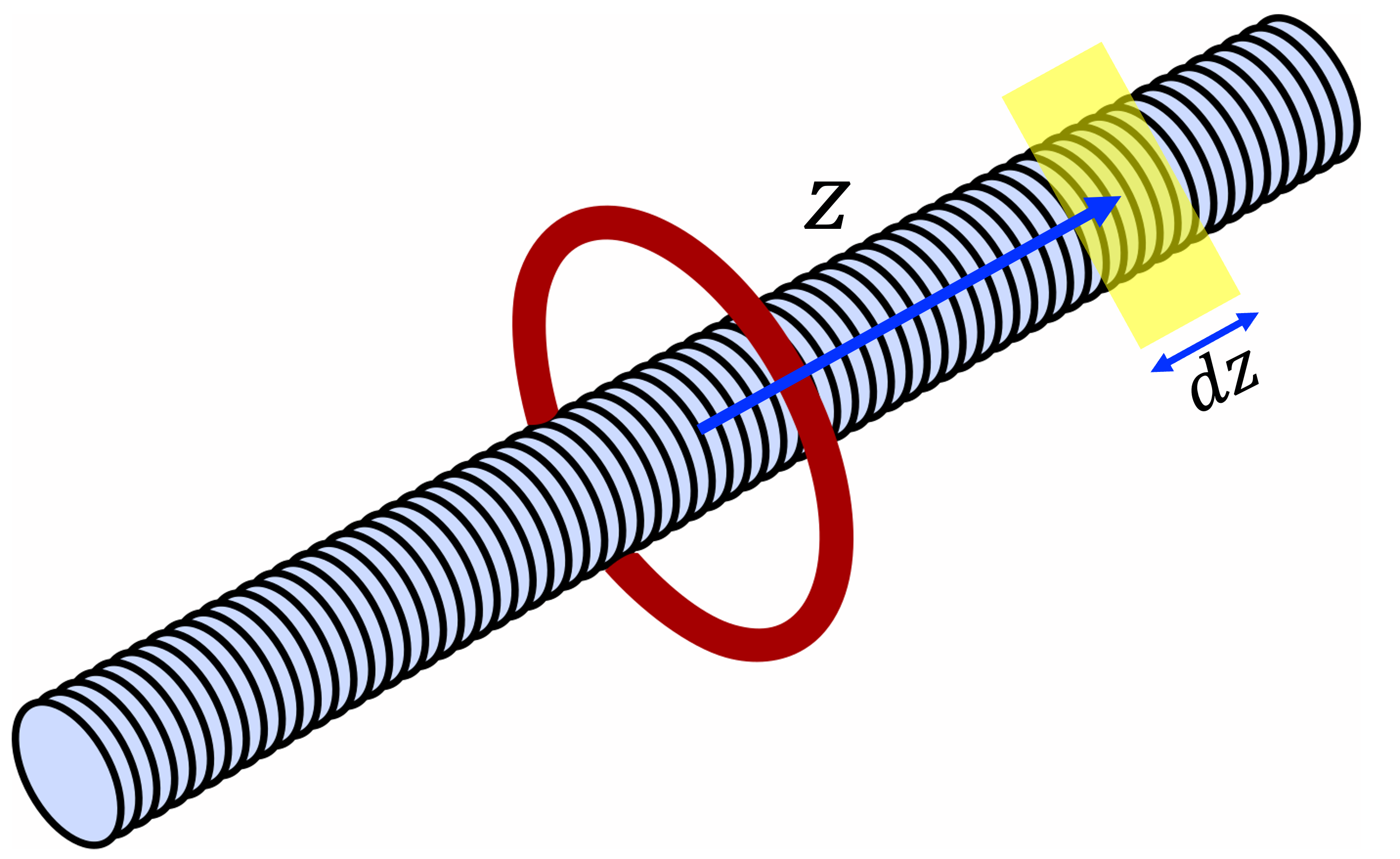
A thin coil with many turns wrapping around a solenoid.
Guy vandegrift, Public domain, via Wikimedia Commons
A thin coil of radius $R_1$ with $N_1$ turns wraps around a long thin solenoid of radius $R_2$ with turns density $n_2$. Assume the coil and the solenoid carry current $I_1$ and $I_2$ respectively. We would use this example to show $M_{12} = M_{21}$ explicitly.
We will need the following two results proven in an earlier chapter with Biot-Savart law:
The magnetic field produced by a coil with $N$ turns along the axis at distance $z$ is $B = \frac{\mu_0 N I R^2 }{2 (z^2 + R^2)^{3/2}}$.
The magnetic field produced by a long solenoid is $B = \mu_0 n I$.
Calculate $\Phi_{12}$, i.e. the magnetic flux picked up by the coil due to the magnetic field of the solenoid.
Calculate $M_{12}$.
Calculate $d\Phi_{21}$, i.e. the small amount of magnetic flux picked up by a section of the solenoid of length $dz$ due to the magnetic field of the coil.
Integrate $d\Phi_{21}$ to find $\Phi_{21}$.
Calculate $M_{21}$.
Solution
$\Phi_{12}$
The magnetic field produced by the solenoid is $B_2 = \mu_0 n_2 I_2$, and this field only exists inside the solenoid, so the total flux captured by the coil is:
$$
\begin{eqnarray}
\Phi_{12} &=& N_1 B_2 A_2 \qquad \text{where $A_2 = \pi R_2^2$} \\
&=& N_1 (\mu_0 n_2 I_2) A_2 \\
&=& \mu_0 N_1 n_2 A_2 I_2
\end{eqnarray}
$$
$d\Phi_{21}$ is the flux captured by the parts of the solenoid highlighted, which consists of $dN_2 = n_2 dz$ turns.
$\Phi_{21}$ is much harder to find, because different parts of the solenoid experience different strength of $B_1$ from the coil. More specifically, the larger $z$ is the weaker $B_1$ becomes, so the sections of the solenoid further away contribute less to $\Phi_{21}$.
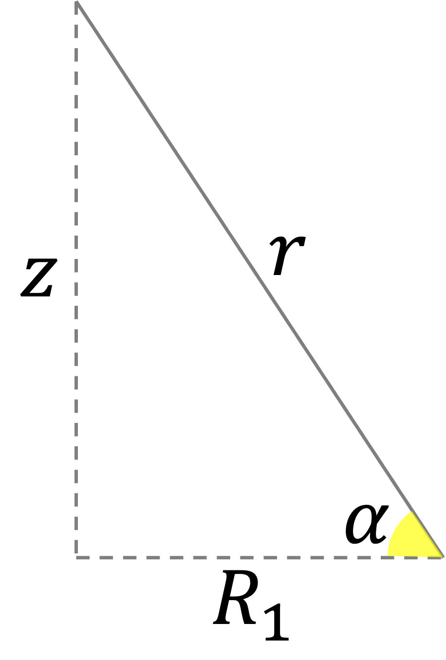
To account for this, we consider only a small section of the solenoid with length $dz$ (see figure), at distance $z$ from the coil, and calculate the magnetic flux picked up by only this section. At this location, the magnetic field produced by the coil is given by $B_1 = \frac{\mu_0 N_1 I_1 R_1^2 }{2 (z^2 + R_1^2)^{3/2}}$. The number of turns of the solenoid within $dz$ is $dN_2 = n_2 dz$. This gives the flux picked up by this section:
$$
\begin{eqnarray}
d\Phi_{21} &=& dN_2 B_1 A_2 \\
&=& (n_2 dz)(\frac{\mu_0 N_1 I_1 R_1^2 }{2 (z^2 + R_1^2)^{3/2}}) A_2 \\
&=& \frac{1}{2} \mu_0 N_1 n_2 A_2 I_1 R_1^2 \frac{dz}{(z^2 + R_1^2)^{3/2}}
\end{eqnarray}
$$
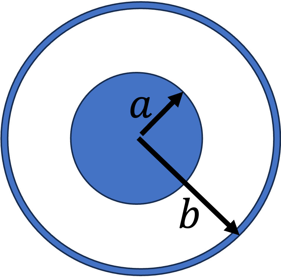
Cross section of a coaxial cable where $I$ points out of the screen in the inner wire, but into the screen in the outer cylinder.
A coaxial cable of length $l$ consists of a solid thick wire of radius $a$, surrounded by a hollow cylinder of radius $b$ (of negligible thickness), carrying current $I$ in opposite directions, coming out of the screen in the inner wire but into the screen in the outer cylinder. Unlike the chapter on Ampere's law, here we assume (for simplicity) the current $I$ on the inner wire is flowing on the wire's surface alone. This allows us to ignore the magnetic field inside at $r \lt a$. Express your answers below in terms of $\mu_0$, $I$, $a$, $b$, and $l$.
Find the magnetic field in the middle region $a \lt r \lt b$ using Ampere's law.
Calculate the total magnetic flux in the coaxial cable.
Calculate the inductance.
Solution
Middle $a \lt r \lt b$
An Amperian loop inside in the counterclockwise direction. $I$ points out of the screen in the inner wire, but into the screen in the outer cylinder.
The Amperian loop shown encloses the entire inner wire, therefore $I_{enclosed} = I$:
$$
\begin{eqnarray}
\mu_0 I &=& \oint \vec B\cdot d\vec s \\
&=& B (2\pi r) \\
\Rightarrow B_{middle} &=& \frac{\mu_0 I}{2\pi r}
\end{eqnarray}
$$
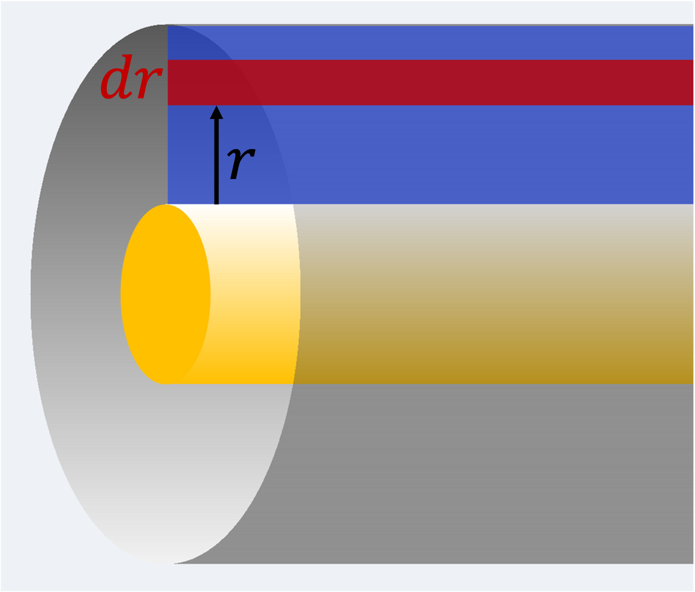
Magnetic flux
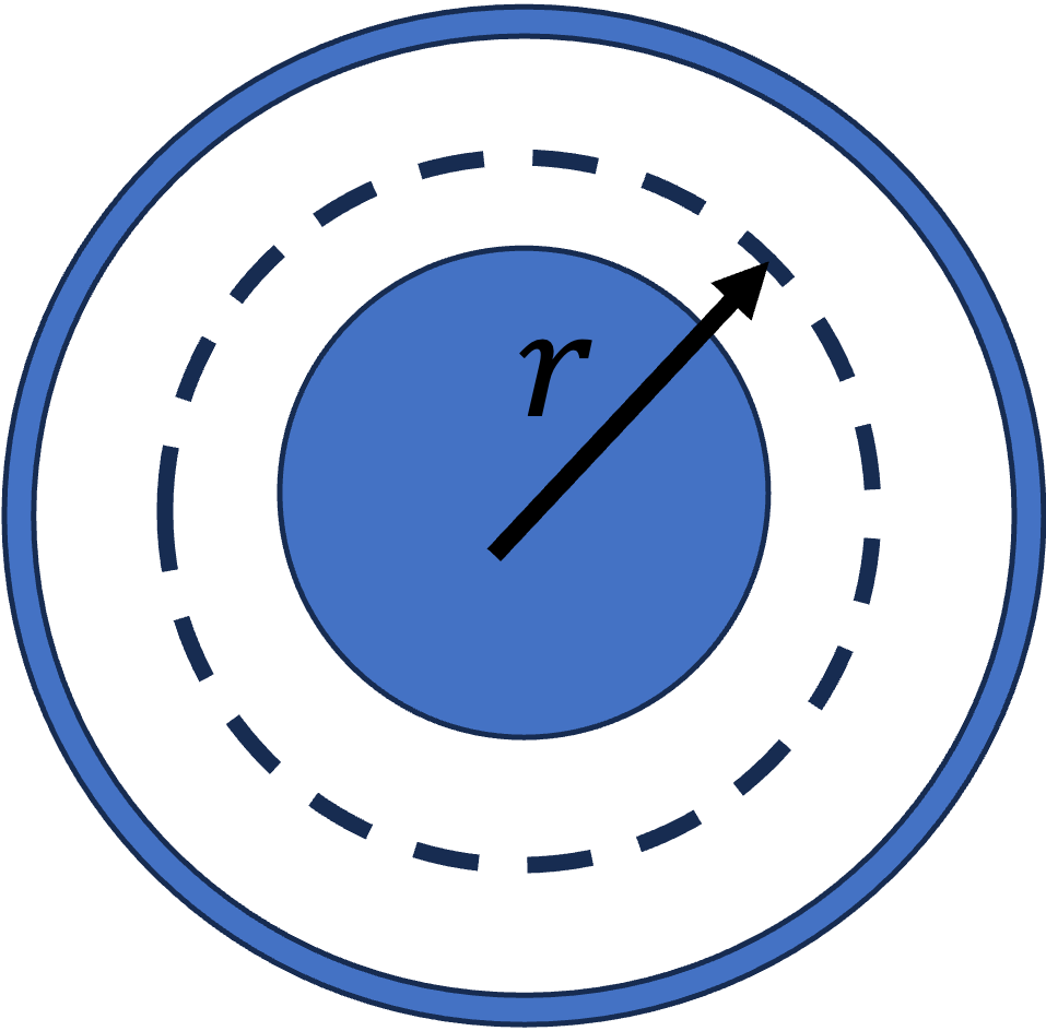
The area through which the magnetic flux is captured. We need to integrate over $r$. An area element is $dA = l dr$.
To calculate the flux, first you should recognize the magnetic field lines are circular and wraps around the inner wire. The area that $\vec B$ crosses is highlighted in blue in the figure. You may be tempted to say $\Phi = BA$, however, since $B$ depends on $r$, integration is required.
For the flux in the region $a \lt r \lt b$, we have:
$$
\begin{eqnarray}
\Phi &=& \int \vec B\cdot d\vec A = \int B dA \\
&=& \int_a^b \frac{\mu_0 I}{2\pi r} (l dr) \\
&=& \frac{\mu_0 I l}{2\pi} \int_a^b \frac{dr}{r} \\
&=& \frac{\mu_0 I l}{2\pi} \ln \frac{b}{a}
\end{eqnarray}
$$
You do not need to know this for the exam, but if you assume the current $I$ is spread evenly across the cross section of the inner wire, the total flux takes quite a bit more work to get because the current is located at different radius $r_1$:
$$
\begin{eqnarray}
\Phi &=& \int_0^a dr_1 \frac{2 r_1}{a^2} \int_{r_1}^b B(r_2) ldr_2 \\
&=& \int_0^a dr_1 \frac{2 r_1}{a^2} \bigg( \int_{r_1}^a B_{in}(r_2) ldr_2 + \int_a^b B_{middle}(r_2) ldr_2 \bigg) \\
&=& \frac{2 }{a^2} \int_0^a r_1 dr_1 \bigg( \int_{r_1}^a \frac{\mu_0 I r_2}{2\pi a^2} ldr_2 + \int_a^b \frac{\mu_0 I}{2\pi r_2} ldr_2 \bigg) \\
&=& \frac{2}{a^2} \int_0^a r_1 dr_1 \bigg( \frac{\mu_0 I l (a^2 - r_1^2)}{4\pi a^2} + \frac{\mu_0 I l}{2\pi} \ln \frac{b}{a} \bigg) \\
&=& \frac{2}{a^2} \int_0^a dr_1 \bigg( \frac{\mu_0 I l (a^2 r_1 - r_1^3)}{4\pi a^2} + r_1 \frac{\mu_0 I l}{2\pi} \ln \frac{b}{a} \bigg) \\
&=& \frac{\mu_0 I l (a^2 \frac{a^2}{2} - \frac{a^4}{4})}{4\pi a^4} + \frac{\mu_0 I l}{2\pi} \ln \frac{b}{a} \\
&=& \frac{\mu_0 I l}{8\pi a^4} + \frac{\mu_0 I l}{2\pi} \ln \frac{b}{a} \\
&=& \frac{\mu_0 I l}{2\pi} (\ln \frac{b}{a} + \frac{1}{4})
\end{eqnarray}
$$
Removing the $\frac{1}{4}$ term give the same answer we had earlier.
Cross section of a coaxial cable where $I$ points out of the screen in the inner wire, but into the screen in the outer cylinder.
A coaxial cable consists of a solid thick wire of radius $a$, surrounded by a hollow cylinder of radius $b$ (of negligible thickness), carrying current $I$ in opposite directions, coming out of the screen in the inner wire but into the screen in the outer cylinder. Unlike the chapter on Ampere's law, here we assume (for simplicity) the current $I$ on the inner wire is flowing on the wire's surface alone. This allows us to ignore the magnetic field inside at $r \lt a$.
Find the magnetic field in the middle region $a \lt r \lt b$.
Write down the expressions of the energy density $u = \frac{1}{2 \mu_0} B^2$ for the middle region.
By integrating over the energy density, find the total magnetic energy $U$ in the coaxial cable. You can use the volume element of cylinderical coordinates $dV = rdr d\theta dz$ to perform the integration.
Calculate the inductance using $U = \frac{1}{2}LI^2$.
So far we have ignored the region $r \lt a$. Suppose the energy carried by the magnetic field by the inner wire is $U_{in} = \frac{\mu_0 I^2 l}{16\pi}$ (proven in Energy density inside a thick wire), find the inductance taking $U_{in}$ into account.
Solution
Middle $a \lt r \lt b$
An Amperian loop inside in the counterclockwise direction. $I$ points out of the screen in the inner wire, but into the screen in the outer cylinder.
The Amperian loop shown encloses the entire inner wire, therefore $I_{enclosed} = I$:
$$
\begin{eqnarray}
\mu_0 I &=& \oint \vec B\cdot d\vec s \\
&=& B (2\pi r) \\
\Rightarrow B_{middle} &=& \frac{\mu_0 I}{2\pi r}
\end{eqnarray}
$$
$$
\begin{eqnarray}
U_{middle} &=& \frac{1}{2}LI^2 \\
\Rightarrow L &=& \frac{2 U}{I^2} \\
&=& \frac{\mu_0 l}{2\pi}\ln \frac{b}{a}
\end{eqnarray}
$$
This is the same $L$ as derived in an earlier example using the definition $L = \frac{\Phi}{I}$.
Side remarks: including $U_{in}$
You do not need to know this for the exam. In the example Energy density inside a thick wire, the energy inside a thick wire is found to be $U_{in} = \frac{\mu_0 I^2 l}{16\pi}$. If this energy is included to account for the energy in the inner wire of the coaxial cable, then the total energy of a coaxial cable would be:
$$
\begin{eqnarray}
U &=& U_{middle} + U_{in} \\
&=& \frac{\mu_0 I^2 l}{4\pi}\ln \frac{b}{a} + \frac{\mu_0 I^2 l}{16\pi} = \frac{1}{2}L I^2 \\
\Rightarrow L &=& \frac{\mu_0 l}{2\pi}\bigg( \ln \frac{b}{a} + \frac{1}{4} \bigg)
\end{eqnarray}
$$
This is the same answer found under the Side remarks of Inductance of a coaxial cable.
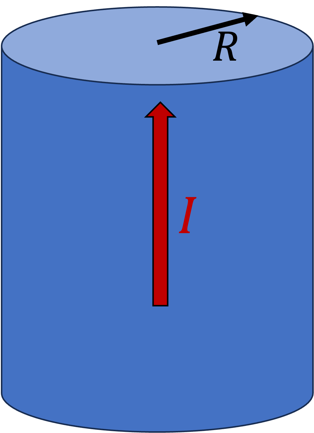
A current $I$ flows through a thick wire with radius $R$. Assume the current is spready evenly throughout the cross-section of the wire.
Find the magnetic field inside $r \lt R$.
Write down the expressions of the energy density $u = \frac{1}{2 \mu_0} B^2$ inside.
By integrating over the energy density, find the magnetic energy $U$ in the region $r \lt R$. You can use the volume element of cylinderical coordinates $dV = rdr d\theta dz$ to perform the integration. You do not need to consider the field outside $r \gt R$.
Solution
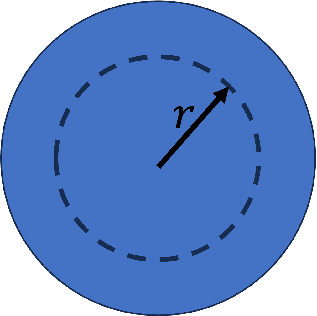
Inside $r \lt R$
An Amperian loop inside in the counterclockwise direction.
The Amperian loop shown encloses only an area $\pi r^2$, which is only part of the entire cross section $\pi R^2$, therefore:
$$
I_{enclosed} = \frac{\pi r^2}{\pi R^2} I = \frac{r^2}{R^2} I
$$
Applying Ampere's law:
$$
\begin{eqnarray}
\mu_0 (\frac{r^2}{R^2} I) &=& \oint \vec B\cdot d\vec s \\
&=& B (2\pi r) \\
\Rightarrow B_{in} &=& \frac{\mu_0 I r}{2\pi R^2}
\end{eqnarray}
$$
For the magnetic energy in the region $r \lt R$, we have:
$$
\begin{eqnarray}
U_{in} &=& \int u_{in} dV \\
&=& \int \frac{\mu_0 I^2 r^2}{8\pi^2 R^4} rdr d\theta dz \\
&=& \frac{\mu_0 I^2}{8\pi^2 R^4}\int_0^R (r^2) rdr \int_0^{2\pi} d\theta \int_0^l dz \\
&=& \frac{\mu_0 I^2}{8\pi^2 R^4}\int_0^R r^3 dr \int_0^{2\pi} d\theta \int_0^l dz \\
&=& \frac{\mu_0 I^2}{8\pi^2 R^4} \frac{R^4}{4} (2\pi) (l) \\
&=& \frac{\mu_0 I^2 l}{16\pi}
\end{eqnarray}
$$
Note that this energy does not include the magnetic field outside the wire.