Exercise Electric Field

Exercise here can be loaded by html files

electricity || e_field

Exercise - Directions of $\vec E$ for one charge

return 0;
return 0;
if (int_count_times_randomized == 0){ return -20; } else { return random_min_max_precision(-60, 60, -1, false, -0.5, 0.5); }
if (int_count_times_randomized == 0){ return 3; } else { return random_min_max_precision(3, 3, 0); //defined in setup_exercise_all.js. }
if (int_count_times_randomized == 0){ return 30; } else { return random_min_max_precision(0, 350, -1); //defined in setup_exercise_all.js. }
return (true);
An electric charge and an observer.
Read off from the figure the angle the field $\vec E_1$ make with the positive $x$-axis.
namespace_e_field.theta_e_1 = ~theta_r_1~ + ((~q_1~>0)? 0: 180); if (namespace_e_field.theta_e_1>360){ namespace_e_field.theta_e_1 -= 360; }
Hint:
  • $\vec E$ points away from a positive charge, and toward a negative charge.

Solution

$\vec E$ points away from a positive charge, but toward a negative charge. $\vec E$ is always drawn at the location of the observer.
$\theta_E=$
return namespace_e_field.theta_e_1;
return Math.abs(difference_in_angle_normalized(x_user, x_correct, false))<0.2 //>
$^\circ$
electricity || e_field

Exercise - Electric field of one charge (magnitude only)

if (int_count_times_randomized == 0){ return -3; } else { return random_min_max_precision(-3, 3, 0); //defined in setup_exercise_all.js. }
if (int_count_times_randomized == 0){ return -1; } else { return random_min_max_precision(-3, 3, 0); //defined in setup_exercise_all.js. }
if (int_count_times_randomized == 0){ return -20; } else { let q = random_min_max_precision(-60, 60, -1); while(q==0){ q = random_min_max_precision(-60, 60, -1); } return q; }
if (int_count_times_randomized == 0){ return 3; } else { return random_min_max_precision(-3, 3, 0); //defined in setup_exercise_all.js. }
if (int_count_times_randomized == 0){ return 2; } else { return random_min_max_precision(-3, 3, 0); //defined in setup_exercise_all.js. }
return (Math.abs(~~charge_01_x - ~~observer_x)>1 || Math.abs(~~charge_01_y - ~~observer_y)>1);
An electric charge and an observer.
Distance measured in meters.
Reminder $1nC=10^{-9}C$

Calculate the magnitude of the electric field given the sepearation between the charge and the observer is $r = [[return sf_latex(namespace_e_field.r_01)]]m$.

let nsp = namespace_e_field; nsp.r_vector_01 = new Class_Vector(~~observer_x - ~~charge_01_x, ~~observer_y - ~~charge_01_y); nsp.r_hat_vector_01 = nsp.r_vector_01.unit_vector(); nsp.r_01 = nsp.r_vector_01.magnitude; nsp.e_with_sign_01 = 8.99 * ~~charge_01_charge / (nsp.r_01 * nsp.r_01); nsp.e_magnitude_01 = Math.abs(nsp.e_with_sign_01); nsp.e_vector_01 = nsp.r_hat_vector_01.times_scalar(nsp.e_with_sign_01);
Hint:
  • $E = |\vec E| = |\frac{q}{4\pi\epsilon_0 r^2}|$

Solution

$\vec E$, not drawn to scale.
$$ \begin{eqnarray} E = |\vec E| &=& |\frac{q}{4\pi\epsilon_0 r^2}| \\ &=& |\frac{k q}{r^2}| \\ &=& |\frac{(8.99\times 10^{9})(~~charge_01_charge \times 10^{-9})}{[[return namespace_e_field.r_01.toFixed(2)]]^2}| \\ &=& [[return sf_latex(namespace_e_field.e_magnitude_01)]] N/C \end{eqnarray} $$
$|\vec E|=$
return namespace_e_field.e_magnitude_01.toFixed(2);
5%
Select unit for the electric field:
$N$
$C$
$C/m$
$N/C$
$C/N$
$V$
$J$
3
electricity || e_field

Exercise - Electric field for one charge from description

if (int_count_times_randomized == 0){ return 3; } else { return random_min_max_precision(2, 10, 0); //defined in setup_exercise_all.js. }
if (int_count_times_randomized == 0){ return -20; } else { return random_min_max_precision(-60, 60, 0, true, -1, 1); }
if (int_count_times_randomized == 0){ return 3; } else { return random_min_max_precision(0, 7, 0); //defined in setup_exercise_all.js. }
return (true);
A $~charge_01_charge~ nC$ (reminder: $1n = 10^{-9}$) charge is $~r_1~ m$ [[return namespace_e_field.charge_direction_long]] ([[return namespace_e_field.charge_direction_short]]) of you. [You may want to draw a picture to help visualize the situation.]
  1. What is the magnitude of the electric field at your location?
  2. What is the direction of the electric field?
namespace_e_field.array_string_direction_long = ['east', 'northeast', 'north', 'northwest', 'west', 'southwest', 'south', 'southeast']; namespace_e_field.array_string_direction_short = ['E', 'NE', 'N', 'NW', 'W', 'SW', 'S', 'SE']; namespace_e_field.charge_direction_long = namespace_e_field.array_string_direction_long[~int_direction~]; namespace_e_field.charge_direction_short = namespace_e_field.array_string_direction_short[~int_direction~]; namespace_e_field.e_with_sign_01 = 8.99 * ~charge_01_charge~ / (~r_1~ * ~r_1~); namespace_e_field.e_magnitude_01 = Math.abs(namespace_e_field.e_with_sign_01); if (~charge_01_charge~ > 0){ namespace_e_field.string_direction_e_field = namespace_e_field.array_string_direction_short[(~int_direction~ + 4)%8] } else { namespace_e_field.string_direction_e_field = namespace_e_field.charge_direction_short; }
Hint:
Electric field points away from positive charge.
Electric field points toward negative charge.

Solution

E fields pointing [[return (~charge_01_charge~>0)? "away from": "toward"]] the [[return (~charge_01_charge~>0)? "positive": "negative"]] charge.
Magnitude
$$ \begin{eqnarray} E = |\vec E| &=& |\frac{q}{4\pi\epsilon_0 r^2}| \\ &=& |\frac{k q}{r^2}| \\ &=& |\frac{(8.99\times 10^{9})(~charge_01_charge~ \times 10^{-9})}{~r_1~ ^2}| \\ &=& [[return sf_latex(namespace_e_field.e_magnitude_01)]] N/C \end{eqnarray} $$
Direction
Recalls that electric field points away from a positive charge but toward a negative charge. Since the charge here is [[return (~charge_01_charge~>0)? "positive": "negative"]], an arrow pointing [[return (~charge_01_charge~>0)? "away from": "toward"]] the charge gives the direction of [[return namespace_e_field.string_direction_e_field]].
$|\vec E |= $
return sf_math(namespace_e_field.e_magnitude_01)
5%

Direction of $\vec E= $
return namespace_e_field.string_direction_e_field
not_number
(N, E, S, W, NE, NW, SE, or SW)
Select unit for $E$:
$V$
$N$
$N/C$
$J$
2
electricity || e_field

Exercise - Direction of electric force

return 0;
return 0;
if (int_count_times_randomized == 0){ return -20; } else { return random_min_max_precision(-60, 60, -1, false, -0.5, 0.5); }
if (int_count_times_randomized == 0){ return 3; } else { return random_min_max_precision(3, 3, 0); //defined in setup_exercise_all.js. }
if (int_count_times_randomized == 0){ return 30; } else { return random_min_max_precision(0, 350, -1); //defined in setup_exercise_all.js. }
if (int_count_times_randomized == 0){ return +20; } else { return random_min_max_precision(-60, 60, -1, false, -0.5, 0.5); }
return (true);
[[ namespace_e_field.theta_e_1 = ~theta_r_1~ + ((~q_1~>0)? 0: 180); if (namespace_e_field.theta_e_1>360){ namespace_e_field.theta_e_1 -= 360; } namespace_e_field.theta_force = namespace_e_field.theta_e_1 + ((~q_observer~>0)? 0: 180); if (namespace_e_field.theta_force>360){ namespace_e_field.theta_force -= 360; } return ""; ]]
An electric charge and an observer.
Hint:
  • $\vec E$ points away from a positive charge, and toward a negative charge.

Solution

$\vec E$ points away from a positive charge, but toward a negative charge. $\vec E$ is always drawn at the location of the observer.
$\vec F_{21} = q_2 \vec E_1$: force on $q_2$ produced by $q_1$. Like charges repel, opposite charges attract.
$\theta_E=$
return namespace_e_field.theta_e_1;
return Math.abs(difference_in_angle_normalized(x_user, x_correct, false))<0.2 //>
$^\circ$
$\theta_F=$
return namespace_e_field.theta_force;
return Math.abs(difference_in_angle_normalized(x_user, x_correct, false))<0.2 //>
$^\circ$
electricity || e_field

Exercise - Electric force from description

if (int_count_times_randomized == 0){ return 3; } else { return random_min_max_precision(2, 10, 0); //defined in setup_exercise_all.js. }
if (int_count_times_randomized == 0){ return -20; } else { return random_min_max_precision(-60, 60, 0, true, -1, 1); }
if (int_count_times_randomized == 0){ return 3; } else { return random_min_max_precision(0, 7, 0); //defined in setup_exercise_all.js. }
if (int_count_times_randomized == 0){ return -30; } else { return random_min_max_precision(-60, 60, 0, true, -1, 1); }
return (true);
A charge $q_1 = ~charge_01_charge~ nC$ (reminder: $1n = 10^{-9}$) is $~r_1~ m$ [[return namespace_e_field.charge_direction_long]] ([[return namespace_e_field.charge_direction_short]]) of another charge $q_2 = ~charge_02_charge~ nC$. [You may want to draw a picture to help visualize the situation.]
  1. What is the magnitude of the electric field generated by $q_1$ at the location of $q_2$?
  2. What is the direction of the electric field you just calculated?
  3. What is the magnitude of the electric force on $q_2$?
  4. What is the direction of the electric force you just calculated?
Very big or very small numbers can be entered as "1.234e-6" (for $ 1.234\times 10^{-6}$).
namespace_e_field.array_string_direction_long = ['east', 'northeast', 'north', 'northwest', 'west', 'southwest', 'south', 'southeast']; namespace_e_field.array_string_direction_short = ['E', 'NE', 'N', 'NW', 'W', 'SW', 'S', 'SE']; namespace_e_field.charge_direction_long = namespace_e_field.array_string_direction_long[~int_direction~]; namespace_e_field.charge_direction_short = namespace_e_field.array_string_direction_short[~int_direction~]; namespace_e_field.e_with_sign_01 = 8.99 * ~charge_01_charge~ / (~r_1~ * ~r_1~); namespace_e_field.e_magnitude_01 = Math.abs(namespace_e_field.e_with_sign_01); namespace_e_field.force_magnitude_01 = Math.abs(~charge_02_charge~ * namespace_e_field.e_magnitude_01 * 1e-9); if (~charge_01_charge~ > 0){ namespace_e_field.string_direction_e_field = namespace_e_field.array_string_direction_short[(~int_direction~ + 4)%8] } else { namespace_e_field.string_direction_e_field = namespace_e_field.charge_direction_short; } if (~charge_01_charge~ * ~charge_02_charge~ > 0){ namespace_e_field.string_direction_e_force = namespace_e_field.array_string_direction_short[(~int_direction~ + 4)%8] } else { namespace_e_field.string_direction_e_force = namespace_e_field.charge_direction_short; }
Hint:
Electric field points away from positive charge.
Electric field points toward negative charge.

$\vec F = q \vec E$.

Solution

Showing $\vec E_1$ (red arrows) generated by $q_1$. The E fields point [[return (~charge_01_charge~>0)? "away from": "toward"]] the [[return (~charge_01_charge~>0)? "positive": "negative"]] charge $q_1$. The fields generated by $q_2$ is not drawn because it is not needed for the problem.
Showing electric force $\vec F_{21}$ (blue arrow) on $q_2$ generated by $q_1$. Since $q_2$ is [[return (~charge_02_charge~>0)? "positive": "negative"]], $\vec F_{21}$ is [[return (~charge_02_charge~>0)? "parallel": "anti-parallel"]] to $\vec E_1$ (red arrows in the last figure). It also shows the two charges [[return (~charge_01_charge~ * ~charge_02_charge~ >0)? "repelling": "attracting"]] each other
Magnitude of $\vec E$
$$ \begin{eqnarray} E_1 = |\vec E_1| &=& |\frac{q_1}{4\pi\epsilon_0 r^2}| \\ &=& |\frac{k q_1}{r^2}| \\ &=& |\frac{(8.99\times 10^{9})(~charge_01_charge~ \times 10^{-9})}{~r_1~ ^2}| \\ &=& [[return sf_latex(namespace_e_field.e_magnitude_01)]] N/C \end{eqnarray} $$
Direction of $\vec E$
Recalls that electric field points away from a positive charge but toward a negative charge. Since the charge here is [[return (~charge_01_charge~>0)? "positive": "negative"]], an arrow pointing [[return (~charge_01_charge~>0)? "away from": "toward"]] $q_1$ gives the direction of [[return namespace_e_field.string_direction_e_field]].
Magnitude of $\vec F$
$$ \begin{eqnarray} \vec F_{21} &=& q_2 \vec E_1 \\ \Rightarrow F &=& |q_2| |\vec E_1| \\ &=& |~charge_02_charge~ \times 10^{-9} C| |[[return sf_latex(namespace_e_field.e_magnitude_01)]] N/C| \\ &=& [[return sf_latex(namespace_e_field.force_magnitude_01)]] N \end{eqnarray} $$
Direction of $\vec F$

Since $q_2$ is [[return (~charge_02_charge~>0)? "positive": "negative"]], $\vec F_{21} = q_2 \vec E_1$ tells us $\vec F_{21}$ is [[return (~charge_02_charge~>0)? "parallel": "anti-parallel"]] to $\vec E_1$. Since $\vec E_1$ points [[return namespace_e_field.string_direction_e_field]], we have $\vec F_{21}$ points [[return namespace_e_field.string_direction_e_force]].

Alternatively, we can figure out the direction by observing that the two charges [[return (~charge_01_charge~ * ~charge_02_charge~ >0)? "repel": "attract"]] each other since like charges repel, opposite charges attract.

$|\vec E |= $
return sf_math(namespace_e_field.e_magnitude_01)
5%

Direction of $\vec E= $
return namespace_e_field.string_direction_e_field
not_number
(N, E, S, W, NE, NW, SE, or SW)
$|\vec F|= $
return sf_math(namespace_e_field.force_magnitude_01)
5%

Direction of $\vec F =$
return namespace_e_field.string_direction_e_force
not_number
(N, E, S, W, NE, NW, SE, or SW)
Select unit for $E$:
$V$
$N$
$N/C$
$J$
2
Select unit for $F$:
$V$
$N$
$N/C$
$J$
1
electricity || e_field

Exercise - Directions of $\vec E$ and $\vec r$ for one charge

[[ namespace_e_field.theta_e_1 = ~theta_r_1~ + ((~q_1~>0)? 0: 180); if (namespace_e_field.theta_e_1>360){ namespace_e_field.theta_e_1 -= 360; } return ""; ]]
An electric charge and an observer.
return 0;
return 0;
if (int_count_times_randomized == 0){ return -20; } else { let q = random_min_max_precision(-60, 60, -1); while(q==0){ q = random_min_max_precision(-60, 60, -1); } return q; }
if (int_count_times_randomized == 0){ return 3; } else { return random_min_max_precision(3, 3, 0); //defined in setup_exercise_all.js. }
if (int_count_times_randomized == 0){ return 30; } else { return random_min_max_precision(0, 350, -1); //defined in setup_exercise_all.js. }
Hint:
  1. Draw an arrow from the charge to the observer (NEVER the other way around!!!). This is $\vec r$.
  2. $\vec E$ points away from a positive charge, and toward a negative charge.
  3. $\vec r$ and $\vec E$ are either parallel (if $q>0$) or anti-parallel (if $q\lt 0$).

Solution

$\vec r$ always point from the charge to the observer.
$\vec E$ points away from a positive charge, but toward a negative charge. $\vec E$ is always drawn at the location of the observer.

$\theta_r = $
return ~theta_r_1~;
return Math.abs(difference_in_angle_normalized(x_user, x_correct, false))<0.2 //>
$^\circ$
$\theta_E=$
return namespace_e_field.theta_e_1;
return Math.abs(difference_in_angle_normalized(x_user, x_correct, false))<0.2 //>
$^\circ$
electricity || e_field

Exercise - Directions of $\vec E$ and $\vec r$ for two charges

[[ namespace_e_field.theta_e_1 = ~theta_r_1~ + ((~q_1~>0)? 0: 180); if (namespace_e_field.theta_e_1>360){ namespace_e_field.theta_e_1 -= 360; } namespace_e_field.theta_e_2 = ~theta_r_2~ + ((~q_2~>0)? 0: 180); if (namespace_e_field.theta_e_2>360){ namespace_e_field.theta_e_2 -= 360; } return ""; ]]
Two electric charges and an observer.
return 0;
return 0;
if (int_count_times_randomized == 0){ return -1; } else { return (Math.random()>0.5)? 1 : -1; }
if (int_count_times_randomized == 0){ return 3.5; } else { return random_min_max_precision(3.5, 3.5, 0); //defined in setup_exercise_all.js. }
if (int_count_times_randomized == 0){ return 30; } else { return random_min_max_precision(0, 350, -1); //defined in setup_exercise_all.js. }
if (int_count_times_randomized == 0){ return +1; } else { return (Math.random()>0.5)? 1 : -1; }
if (int_count_times_randomized == 0){ return 3.5; } else { return random_min_max_precision(3.5, 3.5, 0); //defined in setup_exercise_all.js. }
if (int_count_times_randomized == 0){ return 90; } else { return random_min_max_precision(0, 350, -1); //defined in setup_exercise_all.js. }
return Math.abs(difference_in_angle_normalized(~theta_r_2~, ~theta_r_1~, false))>10;
Hint:
  1. Draw an arrow from the charge to the observer (NEVER the other way around!!!). This is $\vec r$.
  2. $\vec E$ points away from a positive charge, and toward a negative charge.
  3. $\vec r$ and $\vec E$ are either parallel (if $q>0$) or anti-parallel (if $q\lt 0$).

Solution

$\vec r$ always point from the charge to the observer.
$\vec E$ points away from a positive charge, but toward a negative charge. $\vec E$ is always drawn at the location of the observer.
The main lesson is that the fields $\vec E_1$ and $\vec E_2$ (made by $q_1$ and $q_2$) are indepdent of one another. You can solve this problem as if they are two separate problems, one for $q_1$, another for $q_2$.

$\theta_{r1} = $
return ~theta_r_1~;
return Math.abs(difference_in_angle_normalized(x_user, x_correct, false))<0.2 //>
$^\circ$
$\theta_{E1}$
return namespace_e_field.theta_e_1;
return Math.abs(difference_in_angle_normalized(x_user, x_correct, false))<0.2 //>
$^\circ$
$\theta_{r2} = $
return ~theta_r_2~;
return Math.abs(difference_in_angle_normalized(x_user, x_correct, false))<0.2 //>
$^\circ$
$\theta_{E2}$
return namespace_e_field.theta_e_2;
return Math.abs(difference_in_angle_normalized(x_user, x_correct, false))<0.2 //>
$^\circ$
electricity || e_field

Exercise - $\vec r$ and $\hat r$

An electric charge and an observer.
Distance measured in meters.
Reminder $1nC=10^{-9}C$

Calculate $\vec r$, $r$, and $\hat r$.

if (int_count_times_randomized == 0){ return -3; } else { return random_min_max_precision(-3, 3, 0); //defined in setup_exercise_all.js. }
if (int_count_times_randomized == 0){ return -1; } else { return random_min_max_precision(-3, 3, 0); //defined in setup_exercise_all.js. }
if (int_count_times_randomized == 0){ return -20; } else { let q = random_min_max_precision(-60, 60, -1); while(q==0){ q = random_min_max_precision(-60, 60, -1); } return q; }
if (int_count_times_randomized == 0){ return 3; } else { return random_min_max_precision(-3, 3, 0); //defined in setup_exercise_all.js. }
if (int_count_times_randomized == 0){ return 2; } else { return random_min_max_precision(-3, 3, 0); //defined in setup_exercise_all.js. }
return (Math.abs(~~charge_01_x - ~~observer_x)>1 || Math.abs(~~charge_01_y - ~~observer_y)>1);
Hint:
  1. Draw an arrow from the charge to the observer (NEVER the other way around!!!). This is $\vec r$.
  2. From the picture, you can read off the components of $\vec r$
  3. Calculate the magnitude of $\vec r$. This is $|\vec r|$, which we write simply as $r$ (without the vector symbol at the top).
  4. Compute the unit vector $\hat r = \frac{\vec r}{r}$.

Solution

[[ let nsp = namespace_e_field; nsp.r_vector_01 = new Class_Vector(~~observer_x - ~~charge_01_x, ~~observer_y - ~~charge_01_y); nsp.r_hat_vector_01 = nsp.r_vector_01.unit_vector(); nsp.r_01 = nsp.r_vector_01.magnitude; nsp.e_with_sign_01 = 8.99 * ~~charge_01_charge / (nsp.r_01 * nsp.r_01); nsp.e_magnitude_01 = Math.abs(nsp.e_with_sign_01); nsp.e_vector_01 = nsp.r_hat_vector_01.times_scalar(nsp.e_with_sign_01); return ""; ]]
$\vec r$ vector pointing from the charge to the observer.
Find $\vec r$

Draw an arrow $\vec r$ from the charge $q_1$ all the way to the observer. This is the location of the observer from the charge's perspective.

[[return namespace_math_vector.string_explanation_for_component(~~observer_x - ~~charge_01_x, ~~observer_y - ~~charge_01_y, "r", 0)]]

[[return namespace_math_vector.string_explanation_for_magnitude(~~observer_x - ~~charge_01_x, ~~observer_y - ~~charge_01_y, "r", 2)]]

Find $\hat r$

Dividing $\vec r$ by $r=|\vec r|$ then gives: $$ \begin{eqnarray} \hat r &=& \frac{\vec r}{r} \\ &=& \frac{[[return namespace_e_field.r_vector_01.string_mathjax(0, false)]]}{[[return sf_latex(namespace_e_field.r_01)]]} \\ &=& [[return namespace_e_field.r_hat_vector_01.string_mathjax(2, false)]] \end{eqnarray} $$


$\vec r = ($
return namespace_e_field.r_vector_01.x;
0.2
$\hat i +$
return namespace_e_field.r_vector_01.y;
0.2
$\hat j )m$
$r=|\vec r|=$
return namespace_e_field.r_01.toFixed(2);
0.2
$m$
$\hat r = $
return namespace_e_field.r_hat_vector_01.x.toFixed(2);
0.04
$\hat i +$
return namespace_e_field.r_hat_vector_01.y.toFixed(2);
0.04
$\hat j$
electricity || e_field

Exercise - Electric field from one charge

An electric charge and an observer.
Distance measured in meters.
Reminder $1nC=10^{-9}C$

Calculate the electric field and the related variables below.

if (int_count_times_randomized == 0){ return -3; } else { return random_min_max_precision(-3, 3, 0); //defined in setup_exercise_all.js. }
if (int_count_times_randomized == 0){ return -1; } else { return random_min_max_precision(-3, 3, 0); //defined in setup_exercise_all.js. }
if (int_count_times_randomized == 0){ return -20; } else { let q = random_min_max_precision(-60, 60, -1); while(q==0){ q = random_min_max_precision(-60, 60, -1); } return q; }
if (int_count_times_randomized == 0){ return 3; } else { return random_min_max_precision(-3, 3, 0); //defined in setup_exercise_all.js. }
if (int_count_times_randomized == 0){ return 2; } else { return random_min_max_precision(-3, 3, 0); //defined in setup_exercise_all.js. }
return (Math.abs(~~charge_01_x - ~~observer_x)>1 || Math.abs(~~charge_01_y - ~~observer_y)>1);
Hint:

It is a long calculation. The key is to do it step by step:

  1. Draw an arrow from the charge to the observer (NEVER the other way around!!!). This is $\vec r$.
  2. From the picture, you can read off the components of $\vec r$
  3. Calculate the magnitude of $\vec r$. This is $|\vec r|$, which we write simply as $r$ (without the vector symbol at the top).
  4. Compute the unit vector $\hat r = \frac{\vec r}{r}$.
  5. Compute the value of $\frac{q}{4\pi \epsilon_0 r^2}$. Note that this number could be negative.
  6. Put all the numbers into the equation $\vec E = (\frac{q}{4\pi \epsilon_0 r^2}) \hat r$.

Solution

[[ let nsp = namespace_e_field; nsp.r_vector_01 = new Class_Vector(~~observer_x - ~~charge_01_x, ~~observer_y - ~~charge_01_y); nsp.r_hat_vector_01 = nsp.r_vector_01.unit_vector(); nsp.r_01 = nsp.r_vector_01.magnitude; nsp.e_with_sign_01 = 8.99 * ~~charge_01_charge / (nsp.r_01 * nsp.r_01); nsp.e_magnitude_01 = Math.abs(nsp.e_with_sign_01); nsp.e_vector_01 = nsp.r_hat_vector_01.times_scalar(nsp.e_with_sign_01); return ""; ]]
$\vec r$ vector pointing from the charge to the observer.
$\vec E$, not drawn to scale.
$\vec r$

Draw an arrow $\vec r$ from the charge $q_1$ all the way to the observer. This is the location of the observer from the charge's perspective.

[[return namespace_math_vector.string_explanation_for_component(~~observer_x - ~~charge_01_x, ~~observer_y - ~~charge_01_y, "r", 0)]]

$r = |\vec r|$

[[return namespace_math_vector.string_explanation_for_magnitude(~~observer_x - ~~charge_01_x, ~~observer_y - ~~charge_01_y, "r", 2)]]

$\hat r$

Dividing $\vec r$ by $r=|\vec r|$ then gives: $$ \begin{eqnarray} \hat r_1 &=& \frac{\vec r_1}{r_1} \\ &=& \frac{[[return namespace_e_field.r_vector_01.string_latex(2, false)]]}{[[return sf_math(namespace_e_field.r_01)]]} \\ &=& [[return namespace_e_field.r_hat_vector_01.string_mathjax(2, false)]] \end{eqnarray} $$

Use $\vec E = \frac{q}{4\pi\epsilon_0 r^2} \hat r$

First we calculate $\frac{q}{4\pi\epsilon_0 r^2} = \frac{k q}{r^2} = \frac{(8.99\times 10^{9})(~~charge_01_charge \times 10^{-9})}{[[return namespace_e_field.r_01.toFixed(2)]]^2} = [[return namespace_e_field.e_with_sign_01.toFixed(2)]]$.

The $x$ and $y$ components of $\vec E$ are then found by multiplying $\frac{q}{4\pi\epsilon_0 r^2}$ and $ \hat r$ (both we just calculated): $$ \begin{eqnarray} \vec E &=& \frac{q}{4\pi\epsilon_0 r^2} \hat r \\ &=& [[return namespace_e_field.e_with_sign_01.toFixed(2)]] ([[return namespace_e_field.r_hat_vector_01.string_mathjax(2, false)]]) \\ &=& ([[return namespace_e_field.e_vector_01.string_mathjax(2, false)]]) N/C \end{eqnarray} $$

$|\vec E|$

Magnitude of the electric field is given by absolute value of the number we just found earlier. Therefore $|\vec E| = |\frac{q}{4\pi\epsilon_0 r^2} | = |[[return namespace_e_field.e_with_sign_01.toFixed(2) ]]| = [[return namespace_e_field.e_magnitude_01.toFixed(2)]] N/C $.

Alternatively: $$ \begin{eqnarray} |\vec E| &=& \sqrt{([[return sf_latex(namespace_e_field.e_vector_01.x)]])^2 + ([[return sf_latex(namespace_e_field.e_vector_01.y)]])^2} \\ &=& [[return sf_latex(namespace_e_field.e_vector_01.magnitude)]] N/C \end{eqnarray} $$

$\vec r = ($
return namespace_e_field.r_vector_01.x;
0.2
$\hat i +$
return namespace_e_field.r_vector_01.y;
0.2
$\hat j )m$
$r=|\vec r|=$
return namespace_e_field.r_01.toFixed(2);
0.3
$m$
$\hat r = $
return namespace_e_field.r_hat_vector_01.x.toFixed(2);
0.04
$\hat i +$
return namespace_e_field.r_hat_vector_01.y.toFixed(2);
0.04
$\hat j $
$\vec E = $
return namespace_e_field.e_vector_01.x.toFixed(2);
0.5
$\hat i +$
return namespace_e_field.e_vector_01.y.toFixed(2);
0.5
$\hat j$
$|\vec E|=$
return namespace_e_field.e_magnitude_01.toFixed(2);
0.6
Select unit for the electric field:
$N$
$C$
$C/m$
$N/C$
$C/N$
$V$
$J$
3
electricity || e_field

Exercise - Electric field and force of two charges

if (int_count_times_randomized == 0){ return -3; } else { return random_min_max_precision(-3, 3, 0); //defined in setup_exercise_all.js. }
if (int_count_times_randomized == 0){ return -1; } else { return random_min_max_precision(-3, 3, 0); //defined in setup_exercise_all.js. }
if (int_count_times_randomized == 0){ return -20; } else { return random_min_max_precision(-60, 60, -1, false, -1, 1); }
if (int_count_times_randomized == 0){ return 3; } else { return random_min_max_precision(-3, 3, 0); //defined in setup_exercise_all.js. }
if (int_count_times_randomized == 0){ return 2; } else { return random_min_max_precision(-3, 3, 0); //defined in setup_exercise_all.js. }
if (int_count_times_randomized == 0){ return 10; } else { return random_min_max_precision(-60, 60, -1, false, -1, 1); }
if (int_count_times_randomized == 0){ return -1; } else { return random_min_max_precision(-3, 3, 0); //defined in setup_exercise_all.js. }
if (int_count_times_randomized == 0){ return 3; } else { return random_min_max_precision(-3, 3, 0); //defined in setup_exercise_all.js. }
if (int_count_times_randomized == 0){ return -10; } else { let q = random_min_max_precision(-60, 60, -1); return random_min_max_precision(-60, 60, -1, false, -1, 1); }
return ((Math.abs(~~charge_01_x - ~~observer_x)>1 || Math.abs(~~charge_01_y - ~~observer_y)>1) && (Math.abs(~~charge_02_x - ~~observer_x)>1 || Math.abs(~~charge_02_y - ~~observer_y)>1) && (Math.abs(~~charge_01_x - ~~charge_02_x)>1 || Math.abs(~~charge_01_y - ~~charge_02_y)>1)) && !(~~observer_x == ~~charge_01_x && ~~observer_x==~~charge_02_x) && !(~~observer_y == ~~charge_01_y && ~~observer_y==~~charge_02_y);
An electric charge and an observer.
Distance measured in meters.
Reminder $1nC=10^{-9}C$
  1. Calculate the electric field and the related variables below.
  2. If the observer is replaced by a charge $q_3 = ~~charge_03_charge nC$. Find the force $\vec F_3$ on the charge.
Very big or very small numbers can be entered as "1.234e-6" (for $ 1.234\times 10^{-6}$).
let nsp = namespace_e_field; nsp.r_vector_01 = new Class_Vector(~~observer_x - ~~charge_01_x, ~~observer_y - ~~charge_01_y); nsp.r_hat_vector_01 = nsp.r_vector_01.unit_vector(); nsp.r_01 = nsp.r_vector_01.magnitude; nsp.e_with_sign_01 = 8.99 * ~~charge_01_charge / (nsp.r_01 * nsp.r_01); nsp.e_magnitude_01 = Math.abs(nsp.e_with_sign_01); nsp.e_vector_01 = nsp.r_hat_vector_01.times_scalar(nsp.e_with_sign_01); nsp.r_vector_02 = new Class_Vector(~~observer_x - ~~charge_02_x, ~~observer_y - ~~charge_02_y); nsp.r_hat_vector_02 = nsp.r_vector_02.unit_vector(); nsp.r_02 = nsp.r_vector_02.magnitude; nsp.e_with_sign_02 = 8.99 * ~~charge_02_charge / (nsp.r_02 * nsp.r_02); nsp.e_magnitude_02 = Math.abs(nsp.e_with_sign_02); nsp.e_vector_02 = nsp.r_hat_vector_02.times_scalar(nsp.e_with_sign_02); nsp.e_vector_total = nsp.e_vector_01.plus(nsp.e_vector_02); nsp.e_magnitude_total = nsp.e_vector_total.magnitude; nsp.f_3 = nsp.e_vector_total.times_scalar(~~charge_03_charge * 1e-9); nsp.f_3_magnitude = nsp.f_3.magnitude; if (Math.abs(nsp.f_3.x) < 1e-12){ //> nsp.f_3.x = 0; } if (Math.abs(nsp.f_3.y) < 1e-12){ //> nsp.f_3.y = 0; }
Hint:

It is an even longer problem than the one charge problem! However, most of the steps are exactly the same. The key is to do it one charge at a time:

  1. Focus your attention to $q_1$ and the observer. Pretend $q_2$ is not even there.
  2. Repeat the work for the one charge problem to get $\vec r_1$, $r_1=|\vec r_1|$, $\hat r_1$, and $\vec E_1$.
  3. Now focus your attention to $q_2$ and the observer. Pretend $q_1$ is not even there.
  4. Repeat the work for the one charge problem to get $\vec r_2$, $r_2=|\vec r_2|$, $\hat r_2$, and $\vec E_2$.
  5. Add the electric field to get $\vec E_{total} = \vec E_1 + \vec E_2$.
  6. $\vec F_3 = q_3 \vec E_{total}$.

Solution

$\vec r_1$ vector pointing from $q_1$ to the observer.
$\vec E_1$, not drawn to scale.

Calculate $\vec E_1$

$\vec r_1$

Draw an arrow $\vec r_1$ from the charge $q_1$ all the way to the observer. This is the location of the observer from the charge's perspective.

[[return namespace_math_vector.string_explanation_for_component(~~observer_x - ~~charge_01_x, ~~observer_y - ~~charge_01_y, "r_1", 0)]]

$r_1 = |\vec r_1|$

[[return namespace_math_vector.string_explanation_for_magnitude(~~observer_x - ~~charge_01_x, ~~observer_y - ~~charge_01_y, "r_1", 2)]]

$\hat r_1$

Dividing $\vec r_1$ by $r_1=|\vec r_1|$ then gives: $$ \begin{eqnarray} \hat r_1 &=& \frac{\vec r_1}{r_1} \\ &=& \frac{[[return namespace_e_field.r_vector_01.string_latex(2, false)]]}{[[return sf_math(namespace_e_field.r_01)]]} \\ &=& [[return namespace_e_field.r_hat_vector_01.string_mathjax(2, false)]] \end{eqnarray} $$

Use $\vec E_1 = \frac{q_1}{4\pi\epsilon_0 r_1^2} \hat r_1$

First we calculate $\frac{q_1}{4\pi\epsilon_0 r_1^2} = \frac{k q_1}{r_1^2} = \frac{(8.99\times 10^{9})(~~charge_01_charge \times 10^{-9})}{[[return namespace_e_field.r_01.toFixed(2)]]^2} = [[return namespace_e_field.e_with_sign_01.toFixed(2)]]$.

The $x$ and $y$ components of $\vec E_1$ are then found by multiplying $\frac{q_1}{4\pi\epsilon_0 r_1^2}$ and $ \hat r_1$ (both we just calculated): $$ \begin{eqnarray} \vec E_1 &=& \frac{q_1}{4\pi\epsilon_0 r_1^2} \hat r_1 \\ &=& [[return namespace_e_field.e_with_sign_01.toFixed(2)]] ([[return namespace_e_field.r_hat_vector_01.string_mathjax(2, false)]]) \\ &=& ([[return namespace_e_field.e_vector_01.string_mathjax(2, false)]]) N/C \end{eqnarray} $$

Calculate $\vec E_2$

$\vec r_2$

Draw an arrow $\vec r_2$ from the charge $q_2$ all the way to the observer. This is the location of the observer from the charge's perspective.

$\vec r_2$ vector pointing from $q_2$ to the observer.
$\vec E_2$, not drawn to scale.

[[return namespace_math_vector.string_explanation_for_component(~~observer_x - ~~charge_02_x, ~~observer_y - ~~charge_02_y, "r_2", 0)]]

$r_2 = |\vec r_2|$

[[return namespace_math_vector.string_explanation_for_magnitude(~~observer_x - ~~charge_02_x, ~~observer_y - ~~charge_02_y, "r_2", 2)]]

$\hat r_2$

Dividing $\vec r_2$ by $r_2=|\vec r_2|$ then gives: $$ \begin{eqnarray} \hat r_2 &=& \frac{\vec r_2}{r_2} \\ &=& \frac{[[return namespace_e_field.r_vector_02.string_latex(2, false)]]}{[[return sf_math(namespace_e_field.r_02)]]} \\ &=& [[return namespace_e_field.r_hat_vector_02.string_mathjax(2, false)]] \end{eqnarray} $$

Use $\vec E_2 = \frac{q_2}{4\pi\epsilon_0 r_2^2} \hat r_2$

First we calculate $\frac{q_2}{4\pi\epsilon_0 r_2^2} = \frac{k q_2}{r_2^2} = \frac{(8.99\times 10^{9})(~~charge_02_charge \times 10^{-9})}{[[return namespace_e_field.r_02.toFixed(2)]]^2} = [[return namespace_e_field.e_with_sign_02.toFixed(2)]]$.

The $x$ and $y$ components of $\vec E_2$ are then found by multiplying $\frac{q_2}{4\pi\epsilon_0 r_2^2}$ and $ \hat r_2$ (both we just calculated): $$ \begin{eqnarray} \vec E_2 &=& \\ &=& \frac{q_2}{4\pi\epsilon_0 r_2^2} \hat r_2 \\ &=& [[return namespace_e_field.e_with_sign_02.toFixed(2)]] ([[return namespace_e_field.r_hat_vector_02.string_mathjax(2, false)]]) \\ &=& ([[return namespace_e_field.e_vector_02.string_mathjax(2, false)]]) N/C \end{eqnarray} $$

Calculate $\vec E_{total}$

$\vec E_{total} = \vec E_1 + \vec E_2$, not drawn to scale.

Finally, we add the two electric field vectors together to get the total field: $$ \begin{eqnarray} \vec E_{total} &=& \vec E_1 + \vec E_2 \\ &=& ([[return namespace_e_field.e_vector_01.string_mathjax(2, false)]]) \\ &+& ([[return namespace_e_field.e_vector_02.string_mathjax(2, false)]]) \\ &=& ([[return namespace_e_field.e_vector_total.string_mathjax(2, false)]]) N/C \end{eqnarray} $$

$|\vec E_{total}|$
We can then find the magnitude of $\vec E_{total}$: $$ \begin{eqnarray} |\vec E_{total}| &=& \sqrt{([[return sf_latex(namespace_e_field.e_vector_total.x)]])^2 + ([[return sf_latex(namespace_e_field.e_vector_total.y)]])^2} \\ &=& [[return sf_latex(namespace_e_field.e_vector_total.magnitude)]] N/C \end{eqnarray} $$

Always remember that $|\vec E_{total}| \neq |\vec E_1| + |\vec E_2|$ in general!

$\vec F_3$

$$ \begin{eqnarray} \vec F_3 &=& q_3 \vec E_{total} \\ &=& (~~charge_03_charge \times 10^{-9} C) (([[return namespace_e_field.e_vector_total.string_mathjax(2, false)]]) N/C) \\ &=& ([[return namespace_e_field.f_3.string_mathjax(2, false)]]) N \end{eqnarray} $$
$|\vec F_{3}|$
We can then find the magnitude of $\vec F_{3}$: $$ \begin{eqnarray} |\vec F_3| &=& \sqrt{([[return sf_latex(namespace_e_field.f_3.x)]])^2 + ([[return sf_latex(namespace_e_field.f_3.y)]])^2} N \\ &=& [[return sf_latex(namespace_e_field.f_3_magnitude)]] N \end{eqnarray} $$
$\vec r_1 = ($
return namespace_e_field.r_vector_01.x;
0.2
$\hat i +$
return namespace_e_field.r_vector_01.y;
0.2
$\hat j )m$
$r_1=|\vec r_1|=$
return namespace_e_field.r_01.toFixed(2);
0.3
$m$
$\hat r_1 = $
return namespace_e_field.r_hat_vector_01.x.toFixed(2);
0.04
$\hat i +$
return namespace_e_field.r_hat_vector_01.y.toFixed(2);
0.04
$\hat j $
$\vec E_1 = $
return namespace_e_field.e_vector_01.x.toFixed(2);
0.5
$\hat i +$
return namespace_e_field.e_vector_01.y.toFixed(2);
0.5
$\hat j$


$\vec r_2 = ($
return namespace_e_field.r_vector_02.x;
0.2
$\hat i +$
return namespace_e_field.r_vector_02.y;
0.2
$\hat j )m$
$r_2=|\vec r_2|=$
return namespace_e_field.r_02.toFixed(2);
0.3
$m$
$\hat r_2 = $
return namespace_e_field.r_hat_vector_02.x.toFixed(2);
0.04
$\hat i +$
return namespace_e_field.r_hat_vector_02.y.toFixed(2);
0.04
$\hat j $
$\vec E_2 = $
return namespace_e_field.e_vector_02.x.toFixed(2);
0.5
$\hat i +$
return namespace_e_field.e_vector_02.y.toFixed(2);
0.5
$\hat j$
$\vec E_{total} = $
return namespace_e_field.e_vector_total.x.toFixed(2);
0.7
$\hat i +$
return namespace_e_field.e_vector_total.y.toFixed(2);
0.7
$\hat j$
$|\vec E_{total}|=$
return namespace_e_field.e_magnitude_total.toFixed(2);
0.7
$\vec F_3 = $
return sf_math(namespace_e_field.f_3.x);
5%
$\hat i +$
return sf_math(namespace_e_field.f_3.y);
5%
$\hat j$
$|\vec F_3|=$
return sf_math(namespace_e_field.f_3_magnitude);
0.7
Select unit for the electric field:
$N$
$C$
$C/m$
$N/C$
$C/N$
$V$
$J$
3
Select unit for the electric force:
$N$
$C$
$C/m$
$N/C$
$C/N$
$V$
$J$
0
electricity || e_field

Exercise - Electric force of a pair of charges (magnitude only)

if (int_count_times_randomized == 0){ return -3; } else { return random_min_max_precision(-3, 3, 0); //defined in setup_exercise_all.js. }
if (int_count_times_randomized == 0){ return -1; } else { return random_min_max_precision(-3, 3, 0); //defined in setup_exercise_all.js. }
if (int_count_times_randomized == 0){ return -20; } else { return random_min_max_precision(-60, 60, -1, false, -1, 1); }
if (int_count_times_randomized == 0){ return 3; } else { return random_min_max_precision(-3, 3, 0); //defined in setup_exercise_all.js. }
if (int_count_times_randomized == 0){ return 2; } else { return random_min_max_precision(-3, 3, 0); //defined in setup_exercise_all.js. }
if (int_count_times_randomized == 0){ return 30; } else { return random_min_max_precision(-60, 60, -1, false, -1, 1); }
return (Math.abs(~~charge_01_x - ~~observer_x)>1 || Math.abs(~~charge_01_y - ~~observer_y)>1);
[[ let nsp = namespace_e_field; nsp.r_vector_01 = new Class_Vector(~~observer_x - ~~charge_01_x, ~~observer_y - ~~charge_01_y); nsp.r_hat_vector_01 = nsp.r_vector_01.unit_vector(); nsp.r_01 = nsp.r_vector_01.magnitude; nsp.e_with_sign_01 = 8.99 * ~~charge_01_charge / (nsp.r_01 * nsp.r_01); nsp.e_magnitude_01 = Math.abs(nsp.e_with_sign_01); nsp.e_vector_01 = nsp.r_hat_vector_01.times_scalar(nsp.e_with_sign_01); nsp.f_vector = nsp.e_vector_01.times_scalar(~~observer_charge * 1e-9) return ""; ]]
An electric charge and an observer.
Distance measured in meters.
Reminder $1nC=10^{-9}C$
  1. Calculate $E_1$, the magnitude electric field at the position of the observer.
  2. Suppose the observer is replaced by a charge $q_2 = ~~observer_charge nC$. Find the magnitude of the force $F_{21}$ on $q_2$.
Very big or very small numbers can be entered as "1.234e-6" (for $ 1.234\times 10^{-6}$).
Hint:
  • $E_1 = |\vec E_1| = |\frac{q_1}{4\pi\epsilon_0 r^2}|$.
  • $F_{21} = |q_2 \vec E_1| = |q_2| |E_1| = |\frac{q_1 q_2}{4\pi\epsilon_0 r^2}|$.

Solution

$E_1$
$\vec E_1$, not drawn to scale.
$$ \begin{eqnarray} E_1 = |\vec E_1| &=& |\frac{q_1}{4\pi\epsilon_0 r^2}| \\ &=& |\frac{k q_1}{r^2}| \\ &=& |\frac{(8.99\times 10^{9})(~~charge_01_charge \times 10^{-9})}{[[return namespace_e_field.r_01.toFixed(2)]]^2}| \\ &=& [[return sf_latex(namespace_e_field.e_magnitude_01)]] N/C \end{eqnarray} $$
$F_{21}$
$\vec F_{21}$, not drawn to scale.
$$ \begin{eqnarray} F_{21} &=& |q_2 \vec E_1| \\ &=& |q_2| |\vec E_1| \\ &=& |~~observer_charge \times 10^{-9} C | ([[return sf_latex(namespace_e_field.e_magnitude_01)]] N/C) \\ &=& [[return sf_latex(namespace_e_field.f_vector.magnitude)]] N \end{eqnarray} $$ Alternatively, you could use Coulomb's law: $$ \begin{eqnarray} F_{21} &=& |\frac{q_1 q_2}{4\pi\epsilon_0 r^2}| \\ &=& |\frac{k q_1 q_2}{r^2}| \\ &=& |\frac{(8.99\times 10^{9})(~~charge_01_charge \times 10^{-9})(~~observer_charge \times 10^{-9} C )}{[[return namespace_e_field.r_01.toFixed(2)]]^2}| \\ &=& [[return sf_latex(namespace_e_field.f_vector.magnitude)]] N \end{eqnarray} $$
$E_1=$
return namespace_e_field.e_magnitude_01.toFixed(2);
5%

$F_{21}=$
return sf_math(namespace_e_field.f_vector.magnitude);
5%
Select unit for the electric field:
$N$
$C$
$C/m$
$N/C$
$C/N$
$V$
$J$
3
Select unit for the electric force:
$N$
$C$
$C/m$
$N/C$
$C/N$
$V$
$J$
0
electricity || e_field

Exercise - Zero electric field 1

if (int_count_times_randomized == 0){ return 5; } else { return random_min_max_precision(-20, 20, 0); //defined in setup_exercise_all.js }
if (int_count_times_randomized == 0){ return -20; } else { return random_min_max_precision(-20, 20, 0); //defined in setup_exercise_all.js }
if (int_count_times_randomized == 0){ return 10; } else { return 10; }
return (~q_1~ != ~q_2~ && ~q_1~ * ~q_2~ != 0);
Two charges on the $x$-axis.
There are two charges on the $x$-axis, $q_1 = ~q_1~ C$ at the origin, and $q_2 = ~q_2~ C$ at $x_2= ~x_2~ m$. The electric field $\vec E_1$ and $\vec E_2$ are created by $q_1$ and $q_2$ respectively.
  1. Write down the directions of the fields and whether they are opposite in direction in the regions:
    1. $x\lt 0m$
    2. $ 0m \lt x \lt ~x_2~ m$
    3. $ x \gt ~x_2~ m$
  2. Find the location $x$ where the total electric field vanishes.
  3. Where should one puts a charge $q_3 = -2.5C$ so that there is no force on it?
x_left_or_right = ~x_2~ / (1 - Math.sqrt(Math.abs(~q_2~ / ~q_1~))); x_middle = ~x_2~ / (1 + Math.sqrt(Math.abs(~q_2~ / ~q_1~))); x_zero_field = (~q_1~ * ~q_2~ > 0)? x_middle: x_left_or_right;
Hint: For the total electric field to vanish, it must satisfy two criteria.
  • $\vec E_1$ and $\vec E_2$ must be opposite in direction.
  • $\vec E_1$ and $\vec E_2$ must have the same magnitude, i.e. $|\vec E_1| = |\vec E_2|$.
Where $\vec E_{total} = \vec 0$, a charge will have no force on it due to $\vec F = q \vec E$.

Solution

The directions of the E field created by the two charges (the lengths of the arrows are not proportional to the magnitudes). $\vec E_1$ in black, $\vec E_2$ in green.
Direction of the fields
The direction can be found by drawing a simple diagram and remembering E field always points away from a positive charge but toward a negative charge. See figure.
$\vec E_{total} = 0$ can only happen in a region where $\vec E_1$ and $\vec E_2$ are opposite in direction.
Magnitude of the fields
$\vec E_1$ and $\vec E_2$ must have the same magnitude if they are to cancel each other perfectly. We can find the place $x$ where this is true: $$ \begin{eqnarray} |\vec E_1| &=& |\vec E_2| \\ \Rightarrow |\frac{q_1}{4\pi \epsilon_0 x^2}| &=& |\frac{q_2}{4\pi \epsilon_0 (x-x_2)^2}| \\ \Rightarrow \frac{|q_1|}{x^2} &=& \frac{|q_2|}{(x-x_2)^2} \\ \Rightarrow \frac{(x-x_2)^2}{x^2} &=& \frac{|q_2|}{|q_1|} \\ \Rightarrow \frac{x-x_2}{x} &=& \pm \sqrt{|\frac{q_2}{q_1}|} \\ \Rightarrow 1- \frac{x_2}{x} &=& \pm \sqrt{|\frac{q_2}{q_1}|} \\ \Rightarrow \frac{x_2}{x} &=& 1 \mp \sqrt{|\frac{q_2}{q_1}|} \\ \Rightarrow x &=& \frac{x_2}{1 \mp \sqrt{|\frac{q_2}{q_1}|}} \\ &=& \frac{~x_2~ m }{1 \mp \sqrt{|\frac{~q_2~ C}{~q_1~ C}|}} \\ \Rightarrow x &=& [[return sf_latex(x_left_or_right)]] m \text{ or } x = [[return sf_latex(x_middle)]] m \end{eqnarray} $$ At both locations $\vec E_1$ and $\vec E_2$ have the same magnitude.

Note that $x = [[return sf_latex(x_middle)]] m$ is inside the middle region $0 \lt x \lt ~x_2~ m$ while the other solution $x = [[return sf_latex(x_left_or_right)]] m$ is outside. Choosing the location where the fields are also opposite in direction gives: $$ \begin{eqnarray} x &=& [[return sf_latex(x_zero_field)]] m \end{eqnarray} $$
Zero force
Since $\vec F = q \vec E$, the charge $q_3$ will experience no force if you place it where $\vec E = \vec 0$. Therefore the location is the same as the previous answer, $x = [[return sf_latex(x_zero_field)]] m$.
Direciton: type "l" for left, "r" for right.
Same direction or opposite: type "s" for same, "o" for opposite.

At $x\lt 0$:
Direction of $\vec E_1$ =
return (~q_1~ > 0)? "l" : "r";
not_number
Direction of $\vec E_2$ =
return (~q_2~ > 0)? "l" : "r";
not_number
Same direction or opposite?
return (~q_1~ * ~q_2~ > 0)? "s" : "o";
not_number

At $0 \lt x \lt x_2$:
Direction of $\vec E_1$ =
return (~q_1~ > 0)? "r" : "l";
not_number
Direction of $\vec E_2$ =
return (~q_2~ > 0)? "l" : "r";
not_number
Same direction or opposite?
return (~q_1~ * ~q_2~ < 0)? "s" : "o"; //>
not_number

At $x \gt x_2$:
Direction of $\vec E_1$ =
return (~q_1~ > 0)? "r" : "l";
not_number
Direction of $\vec E_2$ =
return (~q_2~ > 0)? "r" : "l";
not_number
Same direction or opposite?
return (~q_1~ * ~q_2~ > 0)? "s" : "o";
not_number

E field vanishes at $x= $
return sf_math(x_zero_field)
5%
$m$
$q_3$ should be at $x= $
return sf_math(x_zero_field)
5%
$m$
Select unit for $E$:
$J/C$
$C/m$
$C$
$V/m$
3
electricity || e_field

Exercise - Balancing gravity (unknown mass)

if (int_count_times_randomized == 0){ return -5; } else { return random_min_max_precision(-20, 20, 0); //defined in setup_exercise_all.js }
if (int_count_times_randomized == 0){ return 20; } else { return random_min_max_precision(10, 90, 0); //defined in setup_exercise_all.js }
return (~q_1~ != 0);
A stationary charge $q_1 = ~q_1~ C$ is suspended in mid-air by an electric field $|\vec E| = ~e_field_magnitude_1~ N/C$.
  1. Find the magnitude of the electric force on the charge.
  2. Find the mass of the charge.
  3. What is the direction of the E field?
e_force_magnitude_1 = Math.abs(~q_1~) * ~e_field_magnitude_1~; m_1 = e_force_magnitude_1 / 9.8;
Hint: For the charge to be stationary, the following must be true.
  • $\vec F_E = q_1 \vec E_1$ and the weight must be opposite in direction.
  • $\vec F_E = q_1 \vec E_1$ and the weight must have the same magnitude.

Solution

The forces and E field acting on the charge. Note that $\vec F_E$ and $\vec E$ are opposite if $q_1$ is negative.
Electric force (magnitude)
$$ \begin{eqnarray} |\vec F_E| &=& |q_1 \vec E| = |q_1| |\vec E|\\ &=& |~q_1~ C| (~e_field_magnitude_1~ N/C) \\ &=& [[return sf_latex(Math.abs(~q_1~) * ~e_field_magnitude_1~)]] N \end{eqnarray} $$
Mass
For the charge to be stationary, $\vec F_E = q_1 \vec E$ and the weight must have the same magnitude: $$ \begin{eqnarray} mg &=& |\vec F_E| \\ \Rightarrow m &=& \frac{|\vec F_E|}{g} \\ &=& \frac{[[return sf_latex(e_force_magnitude_1)]]N}{9.8 m/s^2} \\ &=& [[return sf_latex(m_1)]] kg \end{eqnarray} $$
Direction of the fields
For the electric force $\vec F_E$ to cancel the weight, $\vec F_E = q_1 \vec E$ must point up.
  • If $q_1 \gt 0$: $\vec F_E$ and $\vec E$ are in the same direction
  • If $q_1 \lt 0$: $\vec F_E$ and $\vec E$ are in the opposite direction
In our case, $q_1$ is [[return (~q_1~ > 0)? "greater": "less"]] than zero, therefore $\vec E$ must point [[return (~q_1~ > 0)? "up": "down"]].
$F_E$ =
return sf_math(e_force_magnitude_1);
5%
$N$
$m$ =
return sf_math(m_1);
5%
$kg$
Direction of $\vec E$ =
return (~q_1~ > 0)? "u" : "d";
not_number
(type "u" for up, "d" for down)
Select unit for $E$:
$J/C$
$C/m$
$C$
$V/m$
3
electricity || e_field

Exercise - Balancing gravity (unknown charge)

if (int_count_times_randomized == 0){ return 5; } else { return random_min_max_precision(2, 20, 0); //defined in setup_exercise_all.js }
if (int_count_times_randomized == 0){ return 20; } else { return random_min_max_precision(10, 100, -1); //defined in setup_exercise_all.js }
if (int_count_times_randomized == 0){ return -1; } else { return (Math.random()>0.5)? -1 : +1; }
return (~e_field_magnitude_1~ != 0);
A $~m_1~ kg$ stationary charge $q_1$ is suspended in mid-air by an [[return (~e_field_sign_1~ > 0)? "upward" : "downward"]] electric field with magnitude $|\vec E| = ~e_field_magnitude_1~ N/C$.
  1. Find the weight on the charge (magnitude only).
  2. Find the charge of the particle (including the sign).
weight_1 = ~m_1~ * 9.8; q_1 = weight_1 / ~e_field_magnitude_1~ * ~e_field_sign_1~;
Hint: For the charge to be stationary, the following must be true.
  • $\vec F_E = q_1 \vec E$ and the weight must be opposite in direction.
  • $\vec F_E = q_1 \vec E$ and the weight must have the same magnitude.

Solution

The forces and E field acting on the charge. Note that $\vec F_E$ and $\vec E$ are opposite if $q_1$ is negative.
Weight
$$ \begin{eqnarray} mg &=& (~m_1~ kg) (9.8 m/s^2) \\ &=& [[return sf_latex(weight_1)]] N \end{eqnarray} $$
Charge
For the charge to be stationary, $\vec F_E = q_1 \vec E$ and the weight must have the same magnitude: $$ \begin{eqnarray} mg &=& |\vec F_E| = |q_1| |\vec E| \\ \Rightarrow |q_1| &=& \frac{mg}{|\vec E|} \\ &=& \frac{[[return sf_latex(weight_1)]]N}{~e_field_magnitude_1~ N/C} \\ &=& [[return sf_latex(Math.abs(q_1))]] C \\ \Rightarrow q_1 &=& \pm [[return sf_latex(Math.abs(q_1))]] C \end{eqnarray} $$ To determine the sign of $q_1$, we note that the electric force $\vec F_E$ cancels the weight, so $\vec F_E$ must point up.
  • If $q_1 \gt 0$: $\vec F_E$ and $\vec E$ are in the same direction
  • If $q_1 \lt 0$: $\vec F_E$ and $\vec E$ are in the opposite direction
Since we know that $\vec E$ points [[return (~e_field_sign_1~ > 0)? "up" : "down"]], i.e. [[return (~e_field_sign_1~ > 0)? "same" : "opposite in"]] direction as $\vec F_E$, it implies the charge must be [[return (~e_field_sign_1~ > 0)? "positive" : "negative"]]: $$ q_1 = [[return sf_latex(q_1)]] C $$
$mg$ =
return sf_math(weight_1);
5%
$N$
$q_1$ =
return sf_math(q_1);
5%
$C$
Select unit for $E$:
$J/C$
$C/m$
$C$
$V/m$
3
electricity || e_field

Exercise - Balancing gravity (unknown E field)

if (int_count_times_randomized == 0){ return 50; } else { return random_min_max_precision(10, 100, 0); //defined in setup_exercise_all.js }
if (int_count_times_randomized == 0){ return -20; } else { return random_min_max_precision(-30, 30, 0); //defined in setup_exercise_all.js }
return (~q_1~ != 0);
A $~m_1~ kg$ stationary charge $q_1 = ~q_1~ C$ is suspended in mid-air by an electric field with magnitude $\vec E$.
  1. Find the weight on the charge (magnitude only).
  2. Find the magnitude of the electric field.
  3. Find the direction of the electric field.
weight_1 = ~m_1~ * 9.8; sign_1 = ~q_1~ / Math.abs(~q_1~); e_field_1 = weight_1 / ~q_1~;
Hint: For the charge to be stationary, the following must be true.
  • $\vec F_E = q_1 \vec E$ and the weight must be opposite in direction.
  • $\vec F_E = q_1 \vec E$ and the weight must have the same magnitude.

Solution

The forces and E field acting on the charge. Note that $\vec F_E$ and $\vec E$ are opposite if $q_1$ is negative.
Weight
$$ \begin{eqnarray} mg &=& (~m_1~ kg) (9.8 m/s^2) \\ &=& [[return sf_latex(weight_1)]] N \end{eqnarray} $$
E field
For the charge to be stationary, $\vec F_E = q_1 \vec E$ and the weight must have the same magnitude: $$ \begin{eqnarray} mg &=& |\vec F_E| = |q_1| |\vec E| \\ \Rightarrow |\vec E| &=& \frac{mg}{|q_1|} \\ &=& \frac{[[return sf_latex(weight_1)]]N}{|~q_1~ C|} \\ &=& [[return sf_latex(Math.abs(e_field_1))]] N/C \end{eqnarray} $$ To determine the direction of $\vec E$, we note that the electric force $\vec F_E$ cancels the weight, so $\vec F_E$ must point up.
  • If $q_1 \gt 0$: $\vec F_E$ and $\vec E$ are in the same direction
  • If $q_1 \lt 0$: $\vec F_E$ and $\vec E$ are in the opposite direction
In our case, $q_1$ is [[return (~q_1~ > 0)? "greater": "less"]] than zero, therefore $\vec E$ must point [[return (~q_1~ > 0)? "up": "down"]].
$mg$ =
return sf_math(weight_1);
5%
$N$
$|\vec E|$ =
return sf_math(Math.abs(e_field_1));
5%

Direction of $\vec E$ =
return (~q_1~ > 0)? "u": "d";
not_number
(type "u" for up, "d" for down)
Select unit for $E$:
$J/C$
$C/m$
$C$
$V/m$
3
electricity || e_field

Exercise - Two charges hanging

if (int_count_times_randomized == 0){ return 0.0015; } else { return random_min_max_precision(0.001, 0.005, 4); //defined in setup_exercise_all.js }
if (int_count_times_randomized == 0){ return 30; } else { return random_min_max_precision(15, 50, 0); //defined in setup_exercise_all.js }
if (int_count_times_randomized == 0){ return 0.02; } else { return 0.02; }
return (true);
Two postive charges hanging and repelling.
Two $m = [[return sf_latex(1000 * ~m_1~)]] g$ balls, each carrying positive charge $q \gt 0C$ are suspended each by a string of length $l = [[return 100 * ~length_1~]] cm$, making a total angle $[[return 2 * ~angle_degree_1~]] ^\circ$ with each other.
  1. What is the separation $s$ between the balls?
  2. By considering the vertical component of the forces, find the tension $T$ in each string.
  3. Find the magnitude of the electric force on each charge.
  4. Find the $q$ in $nC$.
  5. Would the angle change if the sign of the charge is flipped?
  6. Find an expression for $q$ without putting in the numbers (for exam preparation, no online submission).
angle_radian_1 = ~angle_degree_1~ * Math.PI/180; separation_12 = 2 * ~length_1~ * Math.sin(angle_radian_1); weight_1 = ~m_1~ * 9.8; tension_1 = weight_1 / Math.cos(angle_radian_1); force_electric_1 = tension_1 * Math.sin(angle_radian_1); q_1 = Math.sqrt(force_electric_1 / 8.99e9) * separation_12;
Hint: Draw the force diagram of one of the charges. The forces must all cancel out.
  • Balancing the vertical forces gives you $T$.
  • Balancing the horizontal forces gives you $F_E$.
  • Using Coulomb's Law on $F_E$ gives you $q$

Solution

Tension $T$, weight $mg$, and electric force $F_E$.
Note that the three forces must combined to form a closed triangle because $\vec F_{total} = \vec T + \vec W + \vec F_E = \vec 0$ at equilibrium. This shows geometrically why $F_E = mg \tan \theta$.
Separation
The angle with the vertical is half the angle between the strings: $$ \begin{eqnarray} \theta &=& \frac{[[return 2 * ~angle_degree_1~]] ^\circ}{2} \\ &=& ~angle_degree_1~ ^\circ \end{eqnarray} $$ The separation $s$ is twice the distance between the charge and the vertical: $$ \begin{eqnarray} s &=& 2 l \sin \theta \\ &=& 2 (~length_1~ m) \sin ~angle_degree_1~ ^\circ \\ &=& [[return sf_latex(separation_12)]] m \end{eqnarray} $$
Tension
$$ \begin{eqnarray} mg &=& (~m_1~ kg) (9.8 m/s^2) \\ &=& [[return sf_latex(weight_1)]] N \end{eqnarray} $$ The vertical forces must cancel for the charges to be stationary: $$ \begin{eqnarray} \Rightarrow F_{up} &=& F_{down} \\ \Rightarrow T \cos \theta &=& mg \\ \Rightarrow T &=& \frac{mg}{\cos \theta} \\ &=& \frac{[[return sf_latex(weight_1)]] N}{\cos ~angle_degree_1~ ^\circ} \\ &=& [[return sf_latex(tension_1)]] N \end{eqnarray} $$
E force
For the charge to be stationary, $F_E$ (on each charge) must cancel the horizontal compoent of $T$: $$ \begin{eqnarray} F_E &=& T \sin \theta \\ &=& ([[return sf_latex(tension_1)]] N) \sin ~angle_degree_1~ ^\circ \\ &=& [[return sf_latex(force_electric_1)]] N/C \end{eqnarray} $$
Charge
We can find $q$ using Coulomb's law: $$ \begin{eqnarray} F_E &=& \frac{k q^2}{s^2} \\ \Rightarrow q^2 &=& \frac{s^2 F_E}{k} \\ \Rightarrow q &=& s\sqrt{\frac{F_E}{k}} \\ &=& ([[return sf_latex(separation_12)]]m) \sqrt{\frac{[[return sf_latex(force_electric_1)]] N/C}{8.99 \times 10^9 N m^2 / C^2} } \\ &=& [[return sf_latex(q_1)]] C \\ &=& [[return sf_latex(q_1 * 1e9)]] nC \end{eqnarray} $$
Symbolically
$$ \begin{eqnarray} s &=& 2 l \sin \theta \\ T &=& \frac{mg}{\cos \theta} \\ F_E &=& T \sin \theta = \frac{mg \sin \theta}{\cos \theta} = mg \tan \theta \\ q &=& s \sqrt{\frac{F_E}{k}} \\ &=& 2 l \sin \theta \sqrt{\frac{mg \tan \theta}{k}} \end{eqnarray} $$
Separation =
return sf_math(separation_12);
5%
$m$
$T$ =
return sf_math(tension_1);
5%
$N$
$F_E$ =
return sf_math(force_electric_1);
5%
$N$
$q$ =
return sf_math(q_1 * 1e9);
5%
$nC$
Would the angle change if you flip the sign of the charges?
Yes
No
1
electricity || e_field

Exercise - Conducting spheres with charge exchange 1

if (int_count_times_randomized == 0){ return 10; } else { return random_min_max_precision(-20, 20, 0); //defined in setup_exercise_all.js }
if (int_count_times_randomized == 0){ return -16; } else { return random_min_max_precision(-20, 20, 0); //defined in setup_exercise_all.js }
if (int_count_times_randomized == 0){ return 5; } else { return random_min_max_precision(2, 15, 0); //defined in setup_exercise_all.js }
return ((~q_1~ !== ~q_2~) && (~q_1~ * ~q_2~ !== 0) && (~q_1~ + ~q_2~ !== 0) );
Two identical small conducting spheres carrying changes $q_1 = ~q_1~ C$ and $q_2 = ~q_2~ C$ initially experience a force of magnitude $F_{initial} = ~force_initial~ N$ when they are separated by a distance $r$. The two objects are put in contact so the charges are now shared evenly between them. When the sphere are moved back to their original positions, what is the magnitude of the force $F_{final}$ on each sphere now?
q_final = (~q_1~ + ~q_2~)/2; force_final = q_final * q_final / Math.abs(~q_1~ * ~q_2~) * ~force_initial~;
Hint: You can find $r$ in terms of $F_{initial}$. Also using $2q_{final} = q_1 + q_2$, you can calculate the final force.

Solution

The initial force is $F_{initial} = |\frac{q_1 q_2}{4 \pi \epsilon_0 r^2}|$. Rearranging this equation gives: $$ \begin{eqnarray} F_{initial} &=& |\frac{q_1 q_2}{4 \pi \epsilon_0 r^2}| \\ \Rightarrow \frac{1}{4 \pi \epsilon_0 r^2} &=& \frac{F_{initial}}{|q_1 q_2|} \end{eqnarray} $$
After the charges are shared, each sphere now has $q_{final} = \frac{q_1 + q_2}{2} = [[return sf_latex(q_final)]] C$. $$ \begin{eqnarray} F_{final} &=& |\frac{q_{final}^2}{4 \pi \epsilon_0 r^2}| \\ &=& q_{final}^2 \frac{1}{4 \pi \epsilon_0 r^2} \\ &=& q_{final}^2 \frac{F_{initial}}{|q_1 q_2|} \\ &=& ([[return q_final]] C)^2 (\frac{~force_initial~ N }{|(~q_1~ C) (~q_2~ C)|}) \\ &=& [[return sf_latex(force_final)]] N \end{eqnarray} $$
$F_{final}= $
return sf_math(force_final)
5%
Is the force attractive or repulsive?
Attractive
Repulsive
1
Select unit for force:
$V$
$N/C$
$J$
$N$
3
electricity || e_field

Exercise - Charges at the corners of a square (field only)

if (int_count_times_randomized == 0){ return 10; } else { return random_min_max_precision(2, 12, 0); //defined in setup_exercise_all.js }
if (int_count_times_randomized == 0){ return 10; } else { return random_min_max_precision(-20, 20, 0); //defined in setup_exercise_all.js }
if (int_count_times_randomized == 0){ return -12; } else { return random_min_max_precision(-20, 20, 0); //defined in setup_exercise_all.js }
if (int_count_times_randomized == 0){ return 3; } else { return random_min_max_precision(-20, 20, 0); //defined in setup_exercise_all.js }
if (int_count_times_randomized == 0){ return -14; } else { return random_min_max_precision(-20, 20, 0); //defined in setup_exercise_all.js }
return (~q_1~ * ~q_2~ * ~q_3~ * ~q_4~ !== 0);
Four charges on a square of size $l = ~l_1~ m$. Recall $1n = 10^{-9}$.
Four charges are located at the corner of a square measuring $l = ~l_1~ m$ on each side. Recall $1n = 10^{-9}$.
  1. Write down the direction of the E field produced by each charge at the center of the square.
  2. Calculate the distance between each charge from the center of the square.
  3. Calculate the total electric field at the center of the square.
r_1 = ~l_1~ / Math.sqrt(2); e_field_total = new Class_Vector(); e_field_total.x = Math.sqrt(2) * 8.99 * (+(~q_1~) - (~q_2~) - (~q_3~) + (~q_4~)) / (~l_1~ * ~l_1~ ); e_field_total.y = Math.sqrt(2) * 8.99 * (+(~q_1~) + (~q_2~) - (~q_3~) - (~q_4~)) / (~l_1~ * ~l_1~ ); potential_total = 8.99 * (+(~q_1~) + (~q_2~) + (~q_3~) + (~q_4~)) / r_1;
Hint:
  • Use Pythagoras theorem to find the distance to the center.
  • Write down the unit vectors for each charge and simplify before substituting in numbers.

Solution

The right triangle showing the relationship between $r$ and $l$.
Directions of $\vec E$
The directions of $\vec E$ could be found by recalling the field always points away from the positive charges, but toward the negative charges.
The distance to the center
The distance to the center of the square can be found by applying the Pythagoras theorem to the red triangle highlighted in the figure: $$ \begin{eqnarray} l^2 &=& r^2 + r^2 = 2r^2 \\ \Rightarrow r &=& \frac{l}{\sqrt{2}} = \frac{~l_1~ m}{\sqrt{2}} \\ &=& [[return sf_latex(r_1)]] m \end{eqnarray} $$ 
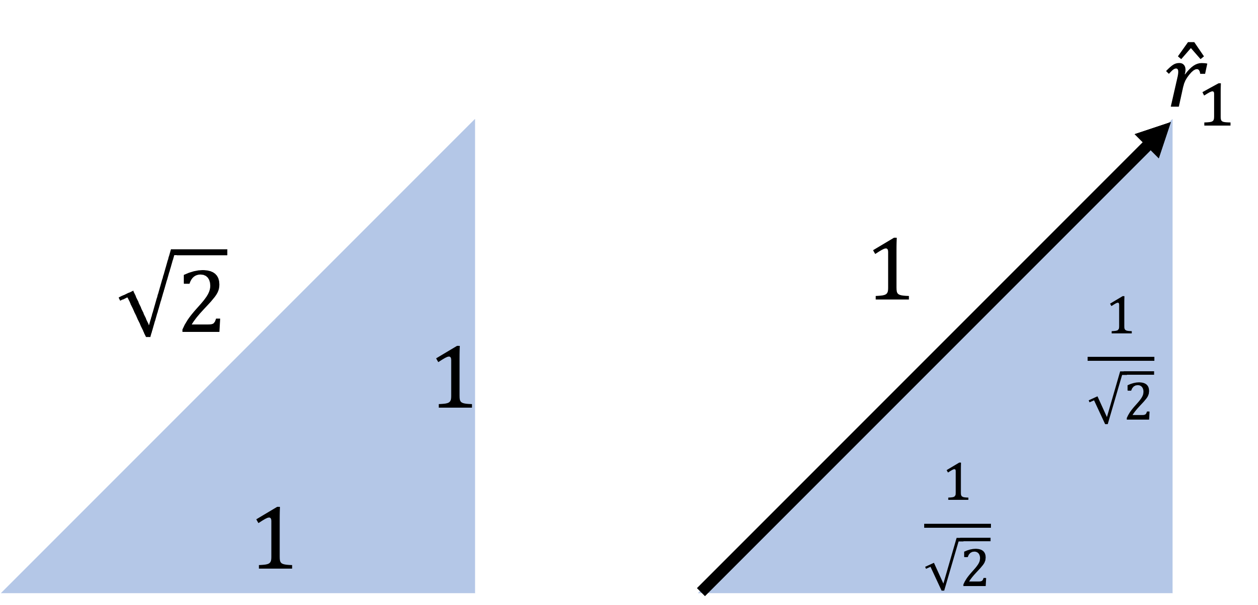
Alternatively, $r = l \cos 45^\circ = l /\sqrt{2}$.
Unit vectors
A standard right triangle at $45^\circ$. Scaling down by $\sqrt{2}$ gives the triangle of length $1$ at the hypotenuse. The vector along the hypotenuse is $\hat r_1$, with both components being $\frac{1}{\sqrt{2}}$. Changing the direction gives the other unit vectors.
The unit vectors for the four charges (which always point away from the charges) can be deduced by the right triangle at $45^\circ$ as shown in the figure: $$ \begin{eqnarray} \hat r_1 &=& \frac{1}{\sqrt{2}}(+\hat i + \hat j) \\ \hat r_2 &=& \frac{1}{\sqrt{2}}(-\hat i + \hat j) \\ \hat r_3 &=& \frac{1}{\sqrt{2}}(-\hat i - \hat j) \\ \hat r_4 &=& \frac{1}{\sqrt{2}}(+\hat i - \hat j) \end{eqnarray} $$ You can check that their magnitudes satisfies $|\hat r| = 1$. This would not be true if the $\frac{1}{\sqrt{2}}$ factor is omitted.
Total E field
$$ \begin{eqnarray} \vec E_{total} &=& \vec E_1 + \vec E_2 + \vec E_3 + \vec E_4 \\ &=& \frac{q_1}{4\pi \epsilon_0 r^2}\hat r_1 + \frac{q_2}{4\pi \epsilon_0 r^2}\hat r_2 + \frac{q_3}{4\pi \epsilon_0 r^2}\hat r_3 + \frac{q_4}{4\pi \epsilon_0 r^2}\hat r_4 \\ &=& \frac{1}{4\pi \epsilon_0 r^2} \frac{1}{\sqrt{2}} \bigg( (+q_1 - q_2 - q_3 + q_4)\hat i + (+q_1 + q_2 - q_3 - q_4)\hat j \bigg) \\ &=& \frac{1}{4\pi \epsilon_0 (\frac{l}{\sqrt{2}})^2} \frac{1}{\sqrt{2}} \bigg( (+q_1 - q_2 - q_3 + q_4)\hat i + (+q_1 + q_2 - q_3 - q_4)\hat j \bigg) \\ &=& (\frac{1}{4\pi \epsilon_0})(\frac{\sqrt{2} }{l^2}) \bigg( (+q_1 - q_2 - q_3 + q_4)\hat i + (+q_1 + q_2 - q_3 - q_4)\hat j \bigg) \\ &=& (8.99\times 10^9 F/m) (\frac{\sqrt{2} }{(~l_1~ m)^2}) \bigg( \big(+(~q_1~) - (~q_2~) - (~q_3~) + (~q_4~)\big)\hat i + \big(+(~q_1~) + (~q_2~) - (~q_3~) - (~q_4~)\big)\hat j \bigg) \times 10^{-9} C \\ &=& ([[return e_field_total.string_mathjax(2, false)]]) V/m \end{eqnarray} $$
Directions of the fields (type "NE", "NW", "SE", or "SW" for northeast, northwest, etc)
$\vec E_1:$
return (~q_1~ > 0)? "NE" : "SW"
not_number
, $\ \vec E_2:$
return (~q_2~ > 0)? "NW" : "SE"
not_number
, $\ \vec E_3:$
return (~q_3~ > 0)? "SW" : "NE"
not_number
, $\ \vec E_4:$
return (~q_4~ > 0)? "SE" : "NW"
not_number

$r = $
return sf_math(r_1)
5%
$m$
$\vec E =$
return sf_math(e_field_total.x)
5%
$\hat i +$
return sf_math(e_field_total.y)
5%
$\hat j$
Select unit for electric field:
$V$
$N/m$
$C/m$
$V/m$
3
electricity || e_field

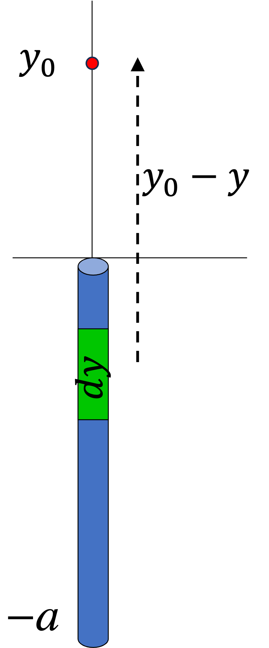
Example - Electric field of a finite bar on the $y$-axis

A bar with uniform linear charge density.
A bar of length $a$ is placed along the negative $y$-axis from the origin to $y=-a$. Charge $Q$ is spread uniformly over the whole bar. An observer is located at point $P$,distance $y_0$ above the origin.
  1. Write down the linear charge density $\lambda$.
  2. Find the amount of charge $dq$ on a line segment of length $dy$ in terms of $\lambda$.
  3. Find the distance $r$ between $P$ and the line segment at $y$.
  4. Write down the magnitude of the E field $dE$ produced by the line segment $dy$ at $P$ in terms of $\lambda$, $y$ and $y_0$.
  5. Integrate $dE$ to find the total field $E$ at $P$ in terms of $Q$, $a$, and $y_0$.
  6. Find $E$ in the limit of $a \rightarrow 0$ (while $Q$ remains constant). What is the physical interpretation of this case?
  7. Find $E$ in the limit of $a \rightarrow \infty$ while keeping $\lambda$ fixed.

Solution

Linear charge density
$$ \lambda = \frac{Q}{a} $$
$dq$
$$ dq = \lambda dy $$
Distance
The distance from $P$ to the line segment: $$ r = y_0 - y $$
$dE$
$$ dE = \frac{dq}{4 \pi \epsilon_0 r^2} = \frac{\lambda dy}{4 \pi \epsilon_0 (y_0 - y)^2} $$
Total electric field
$$ \begin{eqnarray} E &=& \int dE \\ &=& \int_{-a}^0 \frac{\lambda dy}{4 \pi \epsilon_0 (y_0 - y)^2} \\ &=& \frac{\lambda}{4 \pi \epsilon_0} \int_{-a}^0 \frac{ d(y - y_0)}{ (y - y_0)^2} \\ &=& \frac{\lambda}{4 \pi \epsilon_0} (-\frac{1}{y - y_0})\Big|_{y=-a}^{0} \\ &=& \frac{\lambda}{4 \pi \epsilon_0} (\frac{1}{y_0} - \frac{1}{y_0 + a}) \\ &=& \frac{\lambda}{4 \pi \epsilon_0} (\frac{a}{y_0(y_0 + a)}) \\ &=& \frac{Q/a}{4 \pi \epsilon_0} \frac{a}{y_0(y_0 + a)} \\ &=& \frac{Q}{4 \pi \epsilon_0} \frac{1}{y_0(y_0 + a)} \end{eqnarray} $$
The $a \rightarrow 0$ limit while keeping $Q$ fixed
As $a\rightarrow 0$, $E \rightarrow \frac{Q}{4 \pi \epsilon_0 y_0^2}$, which is the expression of the E field produced by a point charge. This is reasonable because as the bar gets shorter and shorter, it becomes more like a point charge at the origin.
The $a \rightarrow \infty$ limit while keeping $\lambda$ fixed
$$ \begin{eqnarray} E &=& \frac{Q}{4 \pi \epsilon_0} \frac{1}{y_0(y_0 + a)} \\ &=& \frac{\lambda a}{4 \pi \epsilon_0} \frac{1}{y_0(y_0 + a)} \\ &\rightarrow& \frac{\lambda a}{4 \pi \epsilon_0} \frac{1}{y_0 a} \\ &=& \frac{\lambda }{4 \pi \epsilon_0 y_0} \end{eqnarray} $$
electricity || e_field

Example - Electric field from an arc (2D)

An arc with radius $R$ and charge $Q$.
A horizontal circular arc with radius $R$ has charge $Q$ spread evenly along its length from $\theta = -\Theta$ to $\theta = +\Theta$.
  1. Find the amount of charge $dq$ on a segment extending by the small angle $d\theta$.
  2. Write down the unit vector $\hat r$ of the segment $dq$.
  3. Write down the E field $d\vec E$ produced by the segment $dq$ at the origin.
  4. Integrate $d\vec E$ to find the total field $\vec E$ at the orgin in terms of $Q$, $R$, and $\Theta$.
  5. Find $\vec E$ in the limit of $\Theta \rightarrow 0$ (while $Q$ remains constant). What is the physical interpretation of this case?
  6. Find $\vec E$ if the arc is a full circle.

Solution

$dq$
$$ dq = \frac{Q}{2\Theta}d\theta $$
$\hat r$
$\hat r$ points from $dq$ to the observer (at the origin), therefore is radially inward: $$ \hat r = -(\cos \theta \hat i + \sin \theta \hat j) $$
$d\vec E$
$$ d\vec E = \frac{dq}{4 \pi \epsilon_0 R^2}\hat r = -\frac{1}{4 \pi \epsilon_0 R^2}\frac{Q}{2\Theta} (\cos \theta \hat i + \sin \theta \hat j) d\theta $$
Total electric field
$$ \begin{eqnarray} \vec E &=& \int d\vec E \\ &=& -\frac{1}{4 \pi \epsilon_0 R^2} \frac{Q}{2\Theta} \int_{-\Theta}^{+\Theta} (\cos \theta \hat i + \sin \theta \hat j) d\theta \\ &=& -\frac{1}{4 \pi \epsilon_0 R^2} \frac{Q}{2\Theta}\bigg( \sin \theta \hat i - \cos \theta \hat j \bigg) \Big|_{-\Theta}^{+\Theta} \\ &=& -\frac{Q}{4 \pi \epsilon_0 R^2} \frac{\sin \Theta}{\Theta} \hat i \end{eqnarray} $$ Note that the $y$-component vanishes as expected by symmetry.
The $\Theta \rightarrow 0$ limit
As $\Theta \rightarrow 0$, $\frac{\sin \Theta}{\Theta}\rightarrow 1$ (you should be able to show this using L'Hôpital's rule), $\vec E \rightarrow -\frac{Q}{4 \pi \epsilon_0 R^2}\hat i$, which is the expression of the E field produced by a point charge. This is reasonable because as the arc gets shorter and shorter, it becomes more like a point charge at the location $x=R$.
Full circle
For a full circle, $\Theta = \pi \Rightarrow \sin \Theta = 0$. This gives $\vec E = \vec 0$. This is expected because of the rotational symmetry of the circle.
electricity || e_field

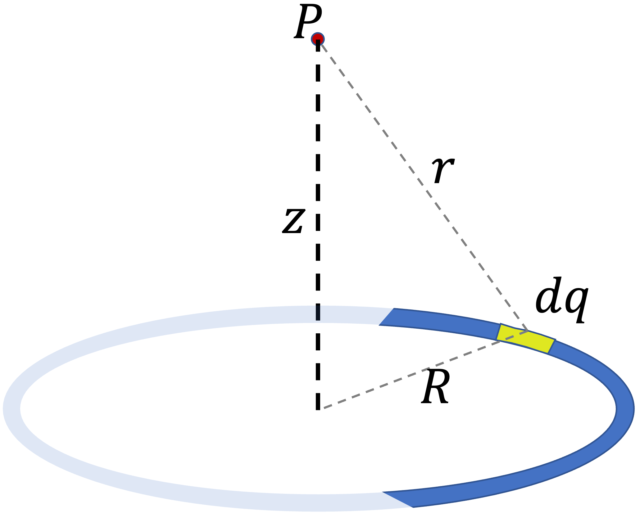
Example - Electric field from an arc (3D)

An arc with radius $R$ and charge $Q$ on the $xy$-plane viewed from above.
The arc viewed in 3d.
A horizontal circular arc with radius $R$ has charge $Q$ spread evenly along its length from $\theta = -\Theta$ to $\theta = +\Theta$. An observer is at point $P$ located at $(0, 0, z)$.
  1. Find the amount of charge $dq$ on a segment extending by the small angle $d\theta$.
  2. Write down the vector $\vec r$ pointing from the segment $dq$ to the observer in terms of $R$, $z$, and $\theta$ (the angle on the $xy$-plane of the arc segment).
  3. Write down the distance $r$ between the segment $dq$ and the observer in terms of $R$, $z$.
  4. Write down the unit vector $\hat r$ of the segment $dq$ in terms of $R$, $z$, and $r$.
  5. Write down the E field $d\vec E$ produced by the segment $dq$ at point $P$ in terms of $Q$, $R$, $\Theta$, $z$, and $r$.
  6. Integrate $d\vec E$ to find the total field $\vec E$ at point $P$ in terms of $Q$, $R$, $z$, and $\Theta$.
  7. Find $\vec E$ if $z=0$.
  8. Find $\vec E$ if the arc is a full circle ($z \neq 0$).
  9. Find $\vec E$ if the arc is a full circle and $R \rightarrow 0$ while $Q$ stays the same. What is the physical interpretation of this case?

Solution

$dq$
$$ dq = \frac{Q}{2\Theta}d\theta $$
$\vec r$
$\vec r$ points from $dq$ to the observer (at the $P$): $$ \vec r = -R\cos \theta \hat i -R \sin \theta \hat j + z \hat k $$
$|\vec r|$
$$ r = |\vec r| = \sqrt{R^2 + z^2} $$
$\hat r$
$$ \hat r = \frac{\vec r}{r} = -\frac{R}{r}\cos \theta \hat i -\frac{R}{r} \sin \theta \hat j + \frac{z}{r} \hat k $$
$d\vec E$
$$ d\vec E = \frac{dq}{4 \pi \epsilon_0 r^2}\hat r = \frac{1}{4 \pi \epsilon_0 r^2}\frac{Q}{2\Theta} (-\frac{R}{r}\cos \theta \hat i -\frac{R}{r} \sin \theta \hat j + \frac{z}{r} \hat k) d\theta $$
Total electric field
$$ \begin{eqnarray} \vec E &=& \int d\vec E \\ &=& \frac{1}{4 \pi \epsilon_0 r^2} \frac{Q}{2\Theta} \int_{-\Theta}^{+\Theta} (-\frac{R}{r}\cos \theta \hat i -\frac{R}{r} \sin \theta \hat j + \frac{z}{r} \hat k) d\theta \\ &=& \frac{1}{4 \pi \epsilon_0 r^2} \frac{Q}{2\Theta}\bigg( -\frac{R}{r}\sin \theta \hat i +\frac{R}{r} \cos \theta \hat j + \frac{z}{r}\theta \hat k \bigg) \Big|_{-\Theta}^{+\Theta} \\ &=& \frac{Q}{4 \pi \epsilon_0 r^2} \bigg( -\frac{R}{r}\frac{\sin \Theta}{\Theta} \hat i + \frac{z}{r} \hat k \bigg) \\ &=& \frac{Q}{4 \pi \epsilon_0 (R^2 + z^2)} \bigg( -\frac{R}{\sqrt{R^2 + z^2}}\frac{\sin \Theta}{\Theta} \hat i + \frac{z}{\sqrt{R^2 + z^2}} \hat k \bigg) \\ \end{eqnarray} $$ Note that the $y$-component vanishes as expected by symmetry.
At $z=0$
At $z=0$, $r = \sqrt{R^2 + z^2} = R$ and $\frac{R}{r} = 1$, so we get: $$ \vec E = -\frac{Q}{4 \pi \epsilon_0 R^2} \frac{\sin \Theta}{\Theta} \hat i $$ This is the same as the answer we obtained in the 2D case earlier.
Full circle
For a full circle, $\Theta = \pi \Rightarrow \sin \Theta = 0$ so the $x$-component vanishes. This gives $\vec E = \frac{Q z}{4 \pi \epsilon_0 r^3} \hat k = \frac{Q z}{4 \pi \epsilon_0 (R^2 + z^2)^{3/2}} \hat k$.
Full circle and $R\rightarrow 0$
In this limit, $r = \sqrt{R^2 + z^2} = z$, therefore: $$ \vec E = \frac{Q z}{4 \pi \epsilon_0 r^3} \hat k = \frac{Q}{4 \pi \epsilon_0 z^2} \hat k $$ This is the same as a point charge $Q$ located at the origin.
electricity || e_field

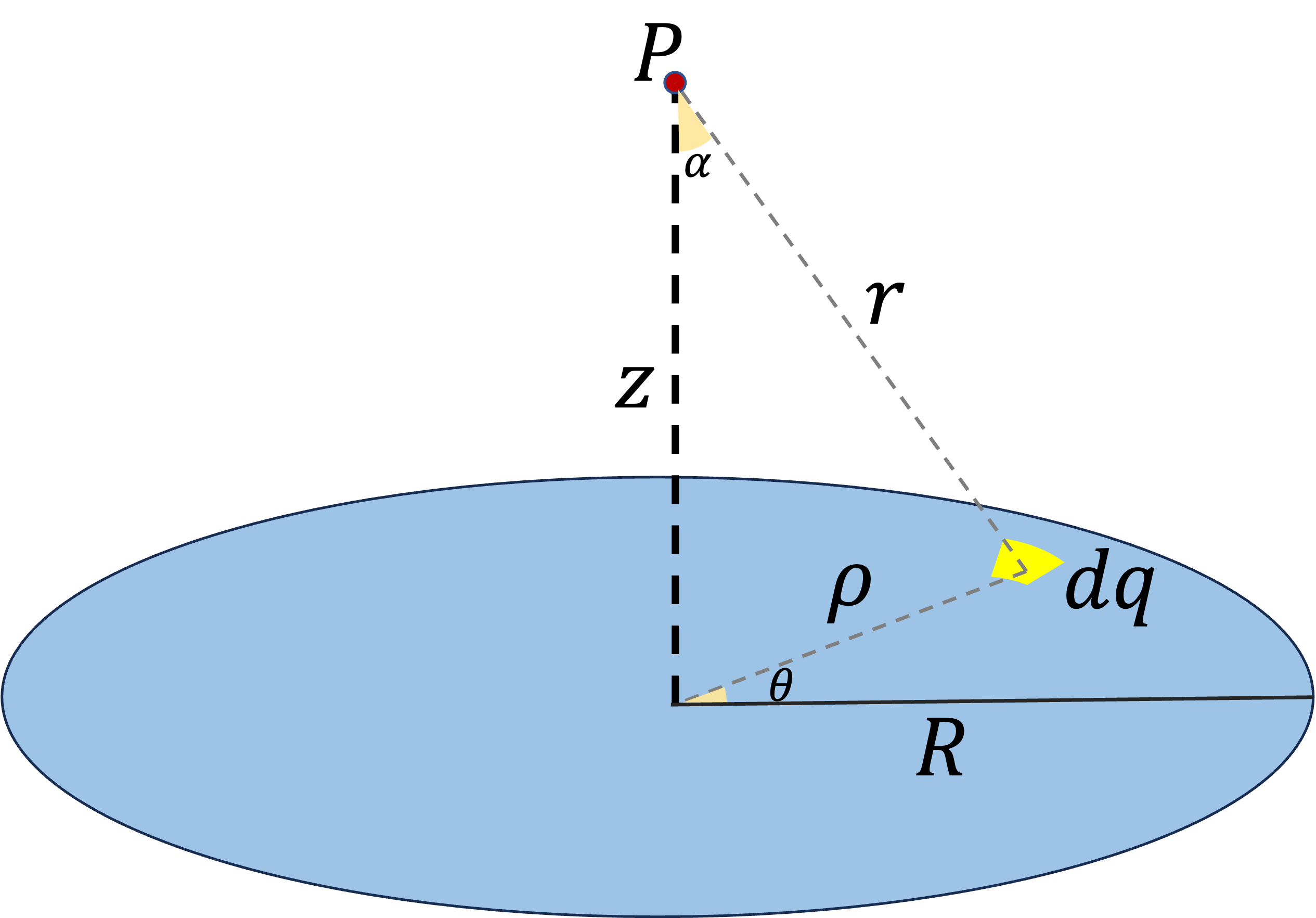
Example - Electric field from a disc (3D)

An disc with radius $R$ and charge $Q$ on the $xy$-plane, with point $P$ directly above the center. $dq$ is the small amount of charge in the highlighted area element.
A horizontal circular disc with radius $R$ has positive charge $Q$ spread evenly over its surface. An observer is at point $P$ located at $(0, 0, z)$. You may use the area element $dA = \rho d\rho d\theta$ for the integration step.
  1. Find the surface charge density $\sigma$ in terms of $Q$ and $R$.
  2. Find the amount of charge $dq$ on an area element extending by the small angle $d\theta$ and radius $d\rho$ in terms of $Q$ and $R$.
  3. Write down the vector $\vec r$ pointing from $dq$ to the observer in terms of $\rho$, $z$, and $\theta$.
  4. Write down the distance $r$ between $dq$ and the observer in terms of $\rho$, $z$.
  5. Write down the unit vector $\hat r$ from $dq$ in terms of $\rho$, $z$, and $r$.
  6. Write down the E field $d\vec E$ produced by $dq$ at point $P$ in terms of $Q$, $\rho$, $z$, and $r$.
  7. Write down the the magnitude $|d\vec E|$ in terms of $Q$, $\rho$, $z$, and $r$.
  8. Integrate $d\vec E$ to find the total field $\vec E$ at point $P$ in terms of $Q$, $R$, and $z$.
  9. Find $E_z$ if $R \rightarrow \infty$ while $\sigma$ stays the same.
  10. Find $E_z$ if $R \rightarrow 0$ while $Q$ stays the same. You may use the approximation $(1+x)^n \approx 1 + nx$ when $x \rightarrow 0$. What is the physical interpretation of this case?

Solution

Surface charge density
$$ \begin{eqnarray} \sigma &=& \frac{Q}{\pi R^2} \end{eqnarray} $$
$dq$
$$ dq = \sigma dA = \frac{Q}{\pi R^2} \rho d\rho d\theta $$
$\vec r$
$\vec r$ points from $dq$ to the observer (at the $P$): $$ \vec r = -\rho\cos \theta \hat i - \rho \sin \theta \hat j + z \hat k $$
$|\vec r|$
$$ r = |\vec r| = \sqrt{\rho^2 + z^2} $$
$\hat r$
$$ \hat r = \frac{\vec r}{r} = -\frac{\rho}{r}\cos \theta \hat i -\frac{\rho}{r} \sin \theta \hat j + \frac{z}{r} \hat k $$
$d\vec E$
$$ d\vec E = \frac{dq}{4 \pi \epsilon_0 r^2}\hat r = \frac{1}{4 \pi \epsilon_0 r^2}\frac{Q}{\pi R^2} (-\frac{\rho}{r}\cos \theta \hat i -\frac{\rho}{r} \sin \theta \hat j + \frac{z}{r} \hat k) \rho d\rho d\theta $$
$|d\vec E|$
$$ |d\vec E| = |\frac{dq}{4 \pi \epsilon_0 r^2}\hat r| = \frac{dq}{4 \pi \epsilon_0 r^2}|\hat r| = \frac{dq}{4 \pi \epsilon_0 r^2} $$
Total electric field
When we integrate over the disc, we expect the $x$ and $y$ components vanish by rotational symmetry, only $E_z$ remains: $$ \begin{eqnarray} dE_z &=& \frac{1}{4 \pi \epsilon_0 r^2}\frac{Q}{\pi R^2} \frac{z}{r} \rho d\rho d\theta \qquad \text{identical to $|d\vec E| \cos \alpha$ because $\cos \alpha = \frac{z}{r}$} \\ \Rightarrow E_z &=& \int dE_z = \int \frac{1}{4 \pi \epsilon_0 r^2}\frac{Q}{\pi R^2} \frac{z}{r} \rho d\rho d\theta \\ &=& \frac{1}{4 \pi \epsilon_0}\frac{Qz}{\pi R^2} \int_0^{2\pi} d\theta \int_0^R \frac{1}{r^3} \rho d\rho \\ &=& \frac{1}{4 \pi \epsilon_0}\frac{Qz}{\pi R^2} (2 \pi) \int_0^R\frac{1}{(\rho^2 + z^2)^{3/2}} \rho d\rho \\ &=& \frac{1}{4 \pi \epsilon_0}\frac{2Qz}{R^2} \int_0^R\frac{1}{(\rho^2 + z^2)^{3/2}} \frac{1}{2} d(\rho^2) \qquad \text{because $d(\rho^2) = 2\rho d\rho$} \\ &=& \frac{1}{4 \pi \epsilon_0}\frac{Qz}{R^2} \int_0^R \frac{1}{(\rho^2 + z^2)^{3/2}} d(\rho^2 + z^2) \qquad \text{because $d(\rho^2 + z^2) = d(\rho^2)$} \\ &=& \frac{1}{4 \pi \epsilon_0}\frac{Qz}{R^2} \frac{-2}{\sqrt{\rho^2 + z^2}}\Bigg|_0^R \qquad \text{because $\int x^{-3/2} dx = -2 x^{-1/2} = \frac{-2}{\sqrt{x}}$} \\ &=& \frac{1}{4 \pi \epsilon_0}\frac{2Qz}{R^2} (\frac{1}{\sqrt{0 + z^2}} - \frac{1}{\sqrt{R^2 + z^2}}) \\ &=& \frac{1}{4 \pi \epsilon_0}\frac{2Qz}{R^2} (\frac{1}{z} - \frac{1}{\sqrt{R^2 + z^2}}) \\ &=& \frac{1}{4 \pi \epsilon_0}\frac{2Q}{R^2} (1 - \frac{z}{\sqrt{R^2 + z^2}}) \tag{1} \end{eqnarray} $$
At $R\rightarrow \infty$ while $\sigma$ stays the same
First we write $Q = \sigma \pi R^2$. In this limit, $\frac{z}{\sqrt{R^2 + z^2}} \rightarrow \frac{z}{R} \rightarrow 0$: $$ \begin{eqnarray} E_z &=& \frac{1}{4 \pi \epsilon_0}\frac{2(\sigma \pi R^2)}{R^2} (1 - \frac{z}{\sqrt{R^2 + z^2}}) \\ &=& \frac{\sigma}{2 \epsilon_0} (1 - \frac{z}{\sqrt{R^2 + z^2}}) \\ &\rightarrow & \frac{\sigma}{2 \epsilon_0} \end{eqnarray} $$ This is the E field produced by an infinite sheet of charge with density $\sigma$, which you will also learn in the chapter on Gauss' law. Note that the E field is no longer dependent on $z$.
$R\rightarrow 0$ while $Q$ stays the same
In this limit: $$ \begin{eqnarray} \frac{z}{\sqrt{R^2 + z^2}} &=& \frac{1}{\sqrt{(\frac{R}{z})^2 + 1}} \\ &=& (1 + (\frac{R}{z})^2)^{-1/2} \\ &\approx & 1 - \frac{1}{2}(\frac{R}{z})^2 \qquad \text{ because $(1+x)^n \approx 1 + nx$ when $x \rightarrow 0$} \\ \Rightarrow 1 - \frac{z}{\sqrt{R^2 + z^2}} &\approx& \frac{1}{2}(\frac{R}{z})^2 \end{eqnarray} $$ Put into (1): $$ \begin{eqnarray} E_z &=& \frac{1}{4 \pi \epsilon_0}\frac{2Q}{R^2} (1 - \frac{z}{\sqrt{R^2 + z^2}}) \\ &\rightarrow& \frac{1}{4 \pi \epsilon_0}\frac{2Q}{R^2} (\frac{1}{2}(\frac{R}{z})^2) \\ &=& \frac{Q}{4 \pi \epsilon_0 z^2} \end{eqnarray} $$ This is the same as the E field created by a point charge $Q$ located at the origin.