if (int_count_times_randomized == 0){
return 2;
} else {
return random_min_max_precision(0.5, 10, 1, true); //defined in setup_exercise_all.js
}
if (int_count_times_randomized == 0){
return 3;
} else {
return random_min_max_precision(0.5, 10, 1, true); //defined in setup_exercise_all.js
}
if (int_count_times_randomized == 0){
return 30;
} else {
return random_min_max_precision(0, 350, -1); //defined in setup_exercise_all.js
}
if (int_count_times_randomized == 0){
return 90;
} else {
return random_min_max_precision(0, 355, 0, true); //defined in setup_exercise_all.js
}
return (true);
Side view of a plane in a uniform electric field. The area vector (not shown) is on the side of the plane that is darkened.
The figure shows the side view of a plane with an area of $ ~area~ m^2$ is placed inside an uniform electric field of $~field~ V/m$. There are two possible choices for the area vector, choose the one on the darkened side.
Find the angle between the area vector and the field. Your answer should be between $0^\circ$ and $180^\circ$.
First draw the area vector perpendicular to the plane, then the angle between $\vec A$ and $\vec B$ can be read off from the diagram to be:
$$
\phi = [[return namespace_gauss.angle_delta]]^\circ
$$
The electric flux is:
$$
\begin{eqnarray}
\Phi &=& E A \cos \phi \\
&=& (~field~ V/m)(~area~ m^2) \cos([[return namespace_gauss.angle_delta]]^\circ) \\
&=& [[return sf_latex(namespace_gauss.flux)]] Vm
\end{eqnarray}
$$
Add up the charges inside the Gaussian surface gives $q_{enclosed} = [[return namespace_gauss.q_enclosed]]C$.
By Gauss' Law:
$$
\Phi = \frac{q_{enclosed}}{\epsilon_0}
= \frac{[[return namespace_gauss.q_enclosed]]C}{8.854\times 10^{-12}F/m}
= [[return get_scientific_notation_latex(namespace_gauss.flux, 2)]] Vm
$$
Note that the unit "Faraday" $F = C/V$, which you will learn in the chapter on capacitance.
Volume of the spherical region:
$$
v = \frac{4}{3}\pi r^3
=\frac{4}{3}\pi ([[return (namespace_gauss.r).toFixed(2)]] m)^3
= [[return (namespace_gauss.v).toFixed(2)]] m^3
$$
Charge enclosed in the shaded region:
$$
q = \rho v = ([[return (namespace_gauss.charge_density).toFixed(2)]] C/m^3)([[return (namespace_gauss.v).toFixed(2)]] m^3)
= [[return (namespace_gauss.charge_enclosed).toFixed(2)]] C
$$
The chosen region encloses the entire sphere, so ALL the charge $Q = ~Q~ C$ is enclosed:
$$
q = [[return (namespace_gauss.charge_enclosed).toFixed(2)]] C
$$
There is no need to use $\rho$ or the volume of the sphere.
Volume of the spherical region that overlaps with the electric charge:
$$
\begin{eqnarray}
v &=& \frac{4}{3}\pi r^3 - \frac{4}{3}\pi a^3 = \frac{4}{3}\pi (r^3 - a^3) \\
&=& \frac{4}{3}\pi (([[return namespace_gauss.r]] m)^3 - ([[return namespace_gauss.a]] m)^3) \\
&=& [[return (namespace_gauss.v).toFixed(2)]] m^3
\end{eqnarray}
$$
Charge enclosed in the shaded region:
$$
q = \rho v = ([[return (namespace_gauss.charge_density).toFixed(2)]] C/m^3)([[return (namespace_gauss.v).toFixed(2)]] m^3)
= [[return (namespace_gauss.charge_enclosed).toFixed(2)]] C
$$
The chosen region encloses the entire shell, so ALL the charge $Q = ~Q~ C$ is enclosed:
$$
q = [[return (namespace_gauss.charge_enclosed).toFixed(2)]] C
$$
There is no need to use $\rho$ or the volume of the shell.
The chosen region is inside the inner radius $a$, so NONE of the charge is enclosed:
$$
q = [[return (namespace_gauss.charge_enclosed).toFixed(2)]] C
$$
There is no need to use $\rho$ or the volume of the shell.
The volume charge density $\rho$ within the shell.
The amount of charge $q$ inside a spherical Gaussian surface of radius $r$.
The total electric flux through the Gaussian surface.
Reminder: $\epsilon_0 = 8.854\times 10^{-12}F/m$.
Very big or very small numbers can be entered as "1.234e-6" (for $ 1.234\times 10^{-6}$).
if (int_count_times_randomized == 0){
return 14;
} else {
let Q = random_min_max_precision(-15, 15, 0); //defined in setup_exercise_all.js
while (Math.abs(Q) < 0.2){ //>
Q = random_min_max_precision(-15, 15, 0);
}
return Q
}
if (int_count_times_randomized == 0){
return 1.1;
} else {
return random_min_max_precision(0.8, 1.5, 2); //defined in setup_exercise_all.js
}
if (int_count_times_randomized == 0){
return 0.8;
} else {
return random_min_max_precision(0.3, 1.2, 1); //defined in setup_exercise_all.js
}
if (int_count_times_randomized == 0){
return 0.5;
} else {
return random_min_max_precision(0.5, 0.8, 2); //defined in setup_exercise_all.js
}
if (int_count_times_randomized == 0){
return -10;
} else {
let Q = random_min_max_precision(-15, 15, 0); //defined in setup_exercise_all.js
while (Math.abs(Q) < 0.2){ //>
Q = random_min_max_precision(-15, 15, 0);
}
return Q
}
Hint:
Account for the absence of charge in the cavity.
$v_{sphere} = \frac{4}{3}\pi r^3$: volume of a sphere
$\rho = \frac{Q}{V} = \frac{q}{v}$: but true only for within the shell that carries electric charge.
$q = \rho v$: where $v$ is the volume that overlaps with the shell.
Solution
Volume of the whole shell:
$$
\begin{eqnarray}
V &=& \frac{4}{3}\pi b^3 - \frac{4}{3}\pi a^3 = \frac{4}{3}\pi (b^3 - a^3) \\
&=& \frac{4}{3}\pi ((~R~ m)^3 - ([[return namespace_gauss.a]] m)^3) \\
&=& [[return (namespace_gauss.V).toFixed(2)]] m^3
\end{eqnarray}
$$
Volume charge density in the shell:
$$
\rho = \frac{Q}{V} = \frac{~Q~ C}{[[return (namespace_gauss.V).toFixed(2)]] m^3}
= [[return (namespace_gauss.charge_density).toFixed(2)]] C/m^3
$$
Volume of the spherical region that overlaps with the electric charge:
$$
\begin{eqnarray}
v &=& \frac{4}{3}\pi r^3 - \frac{4}{3}\pi a^3 = \frac{4}{3}\pi (r^3 - a^3) \\
&=& \frac{4}{3}\pi (([[return namespace_gauss.r]] m)^3 - ([[return namespace_gauss.a]] m)^3) \\
&=& [[return (namespace_gauss.v).toFixed(2)]] m^3
\end{eqnarray}
$$
Charge enclosed in the Gaussian surface:
$$
q = \rho v + q_0 = ([[return (namespace_gauss.charge_density).toFixed(2)]] C/m^3)([[return (namespace_gauss.v).toFixed(2)]] m^3) + (~q_0~ C)
= [[return (namespace_gauss.charge_enclosed).toFixed(2)]] C
$$
The chosen region encloses the entire shell, so ALL the charge $Q + q_0 = ~Q~ C + (~q_0~ C)$ is enclosed:
$$
q = [[return (namespace_gauss.charge_enclosed).toFixed(2)]] C
$$
There is no need to use $\rho$ or the volume of the shell.
The chosen region is inside the inner radius $a$, so only $q_0$ is enclosed:
$$
q = [[return (namespace_gauss.charge_enclosed).toFixed(2)]] C
$$
There is no need to use $\rho$ or the volume of the shell.
The flux can be found simply with Gauss' law:
$$
\Phi = \frac{q_{enclosed}}{\epsilon_0}
= \frac{[[return (namespace_gauss.charge_enclosed).toFixed(2)]]C}{8.854\times 10^{-12}F/m}
= [[return get_scientific_notation_latex(namespace_gauss.flux, 2)]] Vm
$$
Note that the unit "Faraday" $F = C/V$, which you will learn in the chapter on capacitance.
A spherical Gaussian surfrace surrounding a point charge.
By Gauss' law:
$$
\Phi = \frac{q_{enclosed}}{\epsilon_0} = \frac{~Q~ nC}{8.854\times 10^{-12}F/m}
= [[return get_scientific_notation_latex(namespace_gauss.flux, 2)]] Vm
$$
Since it is spherically symmetric, we know the flux is $\Phi = E_r A$. We just calculated the flux from Gauss' law, so we can find the field:
From $E = \frac{|\Phi|}{A} = \frac{|\Phi|}{4\pi r^2}$, substituting in the value for $\Phi$:
$$
\begin{eqnarray}
\Phi &=& E_r A = E_r (4\pi r^2) \\
\Rightarrow E_r &=& \frac{\Phi}{4\pi r^2} \\
&=& \frac{[[return get_scientific_notation_latex(namespace_gauss.flux, 2)]] Vm}{4 \pi (~r~ m)^2} \\
&=& [[return get_scientific_notation_latex(namespace_gauss.e_field, 2)]] V/m
\end{eqnarray}
$$
Symbolically, $\Phi = E_rA=E_r(4\pi r^2)$, and $q_{enclosed} = Q$. Put both into Gauss' law:
$$
\begin{eqnarray}
\Phi &=& \frac{q_{enclosed}}{\epsilon_0} \\
\Rightarrow E_r (4\pi r^2) &=& \frac{Q}{\epsilon_0} \\
\Rightarrow E_r &=& \frac{Q}{4\pi \epsilon_0 r^2}
\end{eqnarray}
$$
A cylindrical Gaussian surface around a line of charge.
A long wire carries a uniform linear charge density $\lambda$. A cylindrical Gaussian surface of length $l$ and radius $r$ is shown surrounding part of the wire.
Charge in a segement:
$$
q = \lambda l = ( ~lambda~ nC/m)( ~l~ m)
= [[return get_scientific_notation_latex(namespace_gauss.charge_enclosed * 1e9, 2)]] nC
$$
$$
\begin{eqnarray}
\Phi_{total} &=& \frac{q_{enclosed}}{\epsilon_0} \\
&=& \frac{[[return get_scientific_notation_latex(namespace_gauss.charge_enclosed * 1e9, 2)]] \times 10^{-9}C}{8.854\times 10^{-12}F/m} \\
&=& [[return get_scientific_notation_latex(namespace_gauss.flux, 2)]] Vm
\end{eqnarray}
$$
Radial electric field (drawn for positive $\lambda$)
Electric field is radial, so none passes through the two caps of the cylinder:
$$
\Phi_{left} = \Phi_{right} = 0Vm
$$
The cylinder consists of three parts, namely the two caps and the curved surface, therefore:
$$
\begin{eqnarray}
\Phi_{total} &=& \Phi_{left} + \Phi_{right} + \Phi_{curved} = 0 + 0 + \Phi_{curved} \\
\Rightarrow \Phi_{curved} &=& \Phi_{total}
= [[return get_scientific_notation_latex(namespace_gauss.flux, 2)]] Vm
\end{eqnarray}
$$
On the curved surface, $d\vec A = dA \hat r$, where $\hat r$ is the cylindrically radial unit vector. Using the same argment as the spherically symmetric case, we can show $\Phi = E_r dA$:
$$
\begin{eqnarray}
\Phi_{curved} &=& \int_{curved} \vec E \cdot d\vec A \\
&=& \int_{curved} \vec E \cdot (dA \hat r) \\
&=& \int_{curved} (\vec E \cdot \hat r) dA \\
&=& \int_{curved} E_r dA & \text{ where $E_r=E \cdot \hat r$ is the cylindrically radial component of the E field}\\
&=& E_r A_{curved}
\end{eqnarray}
$$
The area of the curved surface is:
$$
A_{curved} = 2\pi r l = (2\pi) (~r~ m) (~l~ m)
= [[return get_scientific_notation_latex(namespace_gauss.area, 2)]] m^2
$$
Calculating $E$:
$$
\begin{eqnarray}
E_r A_{curved} &=& \Phi_{curved} \\
\Rightarrow E_r &=& \frac{\Phi_{curved}}{A_{curved}}
= \frac{[[return get_scientific_notation_latex(namespace_gauss.flux, 2)]] Vm}{[[return get_scientific_notation_latex(namespace_gauss.area, 2)]] m^2} \\
&=& [[return get_scientific_notation_latex(namespace_gauss.e_field, 2)]] V/m
\end{eqnarray}
$$
Put both into Gauss' law:
$$
\begin{eqnarray}
\Phi &=& \frac{q_{enclosed}}{\epsilon_0} \\
\Rightarrow E_r (2\pi r l) &=& \frac{\lambda l}{\epsilon_0} \\
\Rightarrow E_r &=& \frac{\lambda}{2\pi \epsilon_0 r}
\end{eqnarray}
$$
You can see from the calculation that $E_r$ does not depend on $l$. Although we used $l = ~l~ m$, $l$ appears once in the numerator (in $q_{enclosed} = \lambda l$) and once in the denominatior (in $A_{curved} = 2\pi r l$), so it cancels out in $E$.
Electric field (drawn for positive $\sigma$) only pierces through the two caps, not the curved surface.
The Gaussian cylinder consists of three surfaces:
Top and bottom caps, each of area $A_{cap} = \pi r^2$.
Curved side, area $A_{curved} = 2\pi r \times (2z)$. Not needed below.
Area of the sheet enclosed by the Gaussian surface is just $A_{cap}$:
$$
A_{cap} = \pi r^2 = \pi ([[return namespace_gauss.r]] m)^2
= [[return sf_latex(namespace_gauss.area_cap)]] m^2;
$$
Charge in the shaded circular region:
$$
q_{enclosed} = \sigma A_{cap} = ([[return (namespace_gauss.charge_density).toFixed(2)]] nC/m^2)([[return sf_latex(namespace_gauss.area_cap)]] m^2)
= [[return (namespace_gauss.charge_enclosed).toFixed(2)]] nC
$$
$$
\begin{eqnarray}
\Phi_{total} &=& \frac{q_{enclosed}}{\epsilon_0} \\
&=& \frac{[[return get_scientific_notation_latex(namespace_gauss.charge_enclosed, 2)]] \times 10^{-9}C}{8.854\times 10^{-12}F/m} \\
&=& [[return get_scientific_notation_latex(namespace_gauss.flux, 2)]] Vm
\end{eqnarray}
$$
The electric field is vertical for an infinite sheet of charge. Therefore the field does not pierce through the curved side of the Gaussian cylinder:
$$
\Phi_{curved} = 0
$$
By symmetry, $\Phi_{top} = \Phi_{bottom}$ (which we will call $\Phi_{cap}$ below), therefore:
$$
\begin{eqnarray}
\Phi_{total} &=& \Phi_{top} + \Phi_{bottom} + \Phi_{curved} = 2\Phi_{cap} \\
\Rightarrow \Phi_{cap} &=& \frac{1}{2} \Phi_{total}
= \frac{[[return sf_latex(namespace_gauss.flux)]] Vm}{2} \\
&=& [[return sf_latex(namespace_gauss.flux/2, 2)]] Vm
\end{eqnarray}
$$
First focus on the top cap, we can show $\Phi_{top} = E_z A$, where $E_z$ is the $z$-component of the E field (perpendicular to the sheet) at the location of the observer.
$$
\begin{eqnarray}
\Phi_{top} &=& \int_{top} \vec E \cdot d\vec A \\
&=& \int_{top} \vec E \cdot (dA \hat k) \\
&=& \int_{top} (\vec E \cdot \hat k) dA \\
&=& \int_{top} E_z dA \\
&=& E_z \int_{top} dA \\
&=& E_z A_{cap}
\end{eqnarray}
$$
Therefore the total flux is:
$$
\begin{eqnarray}
\Phi_{total} &=& \Phi_{top} + \Phi_{bottom} \\
&=& 2 \Phi_{top}\\
&=& 2 E_z A_{cap}
\end{eqnarray}
$$
Solving for $E_z$:
$$
\begin{eqnarray}
\Rightarrow E_z &=& \frac{\Phi_{total}}{2 A_{cap}} \\
&=& \frac{[[return sf_latex(namespace_gauss.flux)]] Vm}{2([[return sf_latex(namespace_gauss.area_cap, 2)]] m^2)} \\
&=& [[return get_scientific_notation_latex(namespace_gauss.e_field, 2)]] V/m
\end{eqnarray}
$$
if (int_count_times_randomized == 0){
return -0.01;
} else {
return random_min_max_precision(-0.01, 0.01, 3, false, -0.004, +0.004); //defined in setup_exercise_all.js
}
if (int_count_times_randomized == 0){
return +0.01;
} else {
return random_min_max_precision(-0.01, 0.01, 3, false, -0.004, +0.004); //defined in setup_exercise_all.js
}
return (true);
Two large sheets of charge with uniform charge density.
Two large sheets with charge density $\sigma_1 = ~density_1~ nC/m^2$ and $\sigma_2 = ~density_2~ nC/m^2$ are placed one above the other.
You may use the equation of the $z$-component of the E field from a large sheet derived earlier. Use the sign to denote the direction of the field (up: $+$, down: $-$).
First consider only sheet 1 (i.e. ignoring sheet 2).
What is $E_{1, above}$, the E field in the region above the sheet?
What is $E_{1, below}$, the E field in the region below the sheet?
Next consider only sheet 2 (i.e. ignoring sheet 1).
What is $E_{2, above}$, the E field in the region above the sheet?
What is $E_{2, below}$, the E field in the region below the sheet?
Now consider both sheets together, sheet 1 above sheet 2.
What is $E_{12, above}$, the E field in the region above both sheets?
What is $E_{12, middle}$, the E field in the region between the sheets?
What is $E_{12, below}$, the E field in the region below both sheets?
Hint:
$E =\frac{\sigma}{2 \epsilon_0}$ for a single sheet.
Combine the fields from the two sheets to get the total field.
The yellow arrows denote the E field of sheet 1, the green arrows that of sheet 2.
The magnitude of the field produced by a sheet of charge is given by $|\vec E|=\frac{|\sigma|}{\epsilon_0}$. The direction can be deduced by the direction of the arrows in the figure (field goes away from positive charges but toward negative charges).
Sheet 1
$$
\begin{eqnarray}
E_{1, above} &=& \pm \frac{|\sigma_1|}{2\epsilon_0} \\
&=& \frac{~density_1~ \times 10^{-9}}{2(8.854\times 10^{-12})} \\
&=& [[return sf_latex(namespace_gauss.field_above_1)]] V/m
\end{eqnarray}
$$
The sign is chosen based on the direction of the yellow arrow above sheet 1.
$$
\begin{eqnarray}
E_{1, below} &=& \pm \frac{|\sigma_1|}{2\epsilon_0} \\
&=& \frac{[[return (-1*~density_1~.toFixed(3))]] \times 10^{-9}}{2(8.854\times 10^{-12})} \\
&=& [[return sf_latex(namespace_gauss.field_below_1)]] V/m
\end{eqnarray}
$$
The sign is chosen based on the direction of the yellow arrow below sheet 1.
Sheet 2
$$
\begin{eqnarray}
E_{2, above} &=& \pm \frac{|\sigma_2|}{2\epsilon_0} \\
&=& \frac{~density_2~ \times 10^{-9}}{2(8.854\times 10^{-12})} \\
&=& [[return sf_latex(namespace_gauss.field_above_2)]] V/m
\end{eqnarray}
$$
The sign is chosen based on the direction of the green arrow above sheet 2.
$$
\begin{eqnarray}
E_{2, below} &=& \pm \frac{|\sigma_2|}{2\epsilon_0} \\
&=& \frac{[[return (-1*~density_2~.toFixed(3))]] \times 10^{-9}}{2(8.854\times 10^{-12})} \\
&=& [[return sf_latex(namespace_gauss.field_below_2)]] V/m
\end{eqnarray}
$$
The sign is chosen based on the direction of the green arrow below sheet 2.
Both sheets
A position above sheet 1 is also above sheet 2, so we have:
$$
\begin{eqnarray}
E_{12, above} &=& E_{1, above} + E_{2, above} \\
&=& ([[return sf_latex(namespace_gauss.field_above_1)]] V/m) + ([[return sf_latex(namespace_gauss.field_above_2)]] V/m) \\
&=& [[return sf_latex(namespace_gauss.field_above_total)]] V/m
\end{eqnarray}
$$
A position in the middle is below sheet 1 but above sheet 2, so we have:
$$
\begin{eqnarray}
E_{12, middle} &=& E_{1, below} + E_{2, above} \\
&=& ([[return sf_latex(namespace_gauss.field_below_1)]] V/m) + ([[return sf_latex(namespace_gauss.field_above_2)]] V/m) \\
&=& [[return sf_latex(namespace_gauss.field_middle_total)]] V/m
\end{eqnarray}
$$
A position below sheet 2 is also below sheet 1, so we have:
$$
\begin{eqnarray}
E_{12, below} &=& E_{1, below} + E_{2, below} \\
&=& ([[return sf_latex(namespace_gauss.field_below_1)]] V/m) + ([[return sf_latex(namespace_gauss.field_below_2)]] V/m) \\
&=& [[return sf_latex(namespace_gauss.field_below_total)]] V/m
\end{eqnarray}
$$
Electric field strength as a function of $r$. Postive value represents field radially outward, negative represents radially inward.
Volume of the spherical region:
$$
v = \frac{4}{3}\pi r^3
=\frac{4}{3}\pi ([[return namespace_gauss.r]] \times 10^{-2} m)^3
= [[return get_scientific_notation_latex(namespace_gauss.v, 2)]] m^3
$$
Charge enclosed in the Gaussian surface:
$$
q_{enclosed} = \rho v = ([[return (namespace_gauss.charge_density)]] nC/m^3)([[return get_scientific_notation_latex(namespace_gauss.v, 2)]] m^3)
= [[return get_scientific_notation_latex(namespace_gauss.charge_enclosed)]] nC
$$
The chosen region encloses the entire sphere, so ALL the charge of the ball is enclosed. Use $R = ~R~ cm$ instead of $r$ to find the volume of the whole ball:
$$
V = \frac{4}{3}\pi R^3
= \frac{4}{3}\pi (~R~ \times 10^{-2} m)^3
= [[return get_scientific_notation_latex(namespace_gauss.V)]] m^3
$$
$$
q_{enclosed} = \rho V = ([[return (namespace_gauss.charge_density)]] nC/m^3)([[return get_scientific_notation_latex(namespace_gauss.V, 2)]] m^3)
= [[return get_scientific_notation_latex(namespace_gauss.charge_enclosed)]] nC
$$
$$
\begin{eqnarray}
\Phi &=& \frac{q_{enclosed}}{\epsilon_0} \\
&=& \frac{[[return get_scientific_notation_latex(namespace_gauss.charge_enclosed, 2)]] \times 10^{-9}C}{8.854\times 10^{-12}F/m} \\
&=& [[return get_scientific_notation_latex(namespace_gauss.flux, 2)]] Vm
\end{eqnarray}
$$
The problem is spherically symmetric, so the flux is given by $\Phi = E_r A$. The area of the Gaussian surface is:
$$
A = 4\pi r^2 = (4\pi) ([[return namespace_gauss.r]] \times 10^{-2} m)^2
= [[return get_scientific_notation_latex(namespace_gauss.area, 2)]] m^2
$$
Calculating $E_r$:
$$
\begin{eqnarray}
E_r &=& \frac{\Phi}{A}
= \frac{[[return get_scientific_notation_latex(namespace_gauss.flux, 2)]] Vm}{[[return get_scientific_notation_latex(namespace_gauss.area, 2)]] m^2} \\
&=& [[return get_scientific_notation_latex(namespace_gauss.e_field, 2)]] V/m
\end{eqnarray}
$$
Electric field strength as a function of $r$. Postive value represents field radially outward, negative represents radially inward.
The Gaussian surface is smaller than the shell, so no charge is enclosed:
$$
q_{enclosed} = 0 nC
$$
$$
\begin{eqnarray}
\Phi &=& \frac{q_{enclosed}}{\epsilon_0} = 0Vm
\end{eqnarray}
$$
$$
\Phi = 0 \Rightarrow E_r = 0V/m
$$
The Gaussian surface encloses the entire sphere, so ALL the charge of the shell is enclosed.
$$
q_{enclosed} = ~Q~ nC
$$
$$
\begin{eqnarray}
\Phi &=& \frac{q_{enclosed}}{\epsilon_0} \\
&=& \frac{[[return get_scientific_notation_latex(namespace_gauss.charge_enclosed, 2)]] \times 10^{-9}C}{8.854\times 10^{-12}F/m} \\
&=& [[return get_scientific_notation_latex(namespace_gauss.flux, 2)]] Vm
\end{eqnarray}
$$
The problem is spherically symmetric, so the flux is given by $\Phi = E_r A$. The area of the Gaussian surface is:
$$
A = 4\pi r^2 = (4\pi) ([[return namespace_gauss.r]] \times 10^{-2} m)^2
= [[return get_scientific_notation_latex(namespace_gauss.area, 2)]] m^2
$$
Calculating $E_r$:
$$
\begin{eqnarray}
E_r &=& \frac{\Phi}{A}
= \frac{[[return get_scientific_notation_latex(namespace_gauss.flux, 2)]] Vm}{[[return get_scientific_notation_latex(namespace_gauss.area, 2)]] m^2} \\
&=& [[return get_scientific_notation_latex(namespace_gauss.e_field, 2)]] V/m
\end{eqnarray}
$$
A spherical Gaussian surface.Electric field strength as a function of $r$. Postive value represents field radially outward, negative represents radially inward.
A few important points:
Charges are free to move in a conductor (such as metal).
Due to their mutual repulsion, charges will all rush to the surface of the sphere.
In the volume of the sphere, there is no charge at all. All charges are found on a very thin layer on the surface.
This problem is the same as the one of a thin spherical shell of charge.
Do not use uniform charge density $\rho$ to do this problem because the density is zero except on the surface of the conducting sphere.
The Gaussian surface is smaller than the sphere, so no charge is enclosed:
$$
q_{enclosed} = 0 nC
$$
$$
\begin{eqnarray}
\Phi &=& \frac{q_{enclosed}}{\epsilon_0} = 0Vm
\end{eqnarray}
$$
$$
\Phi = 0 \Rightarrow E_r = 0V/m
$$
The Gaussian surface encloses the entire sphere, so ALL the charge of the ball is enclosed.
$$
q_{enclosed} = ~Q~ nC
$$
$$
\begin{eqnarray}
\Phi &=& \frac{q_{enclosed}}{\epsilon_0} \\
&=& \frac{[[return get_scientific_notation_latex(namespace_gauss.charge_enclosed, 2)]] \times 10^{-9}C}{8.854\times 10^{-12}F/m} \\
&=& [[return get_scientific_notation_latex(namespace_gauss.flux, 2)]] Vm
\end{eqnarray}
$$
The problem is spherically symmetric, so the flux is given by $\Phi = E_r A$. The area of the Gaussian surface is:
$$
A = 4\pi r^2 = (4\pi) ([[return namespace_gauss.r]] \times 10^{-2} m)^2
= [[return get_scientific_notation_latex(namespace_gauss.area, 2)]] m^2
$$
Calculating $E$:
$$
\begin{eqnarray}
E_r &=& \frac{\Phi}{A}
= \frac{[[return get_scientific_notation_latex(namespace_gauss.flux, 2)]] Vm}{[[return get_scientific_notation_latex(namespace_gauss.area, 2)]] m^2} \\
&=& [[return get_scientific_notation_latex(namespace_gauss.e_field, 2)]] V/m
\end{eqnarray}
$$
A thin shell of charge, uniformly distributed.A spherical Gaussian surface.
An observer is at distance $r$ away from the center of a thin shell of charge (of negligible thickness) with total charge $Q$ and radius $R$. At the center is a point charge $q_0$.
Given:
$Q = ~Q~ nC$ (reminder: $1n = 10^{-9}$)
$q_0 = ~q_0~ nC$
$R = ~R~ cm$ (not in meters!)
$r = [[return namespace_gauss.r]] cm$
Consider a spherical Gaussian surface of radius $r$:
Find the charge enclosed ($q_{enclosed}$).
Find the total flux $\Phi$.
Use Gauss' law to find the radial component of the electric field $E_r$ at the observer's location.
Reminder: $\epsilon_0 = 8.854\times 10^{-12}F/m$.
Very big or very small numbers can be entered as "1.234e-6" (for $ 1.234\times 10^{-6}$).
Hint:
$q_{enclosed} = q_0$ whenever the Gaussian surface is smaller than the shell.
$q_{enclosed} = Q + q_0$ whenever the Gaussian surface is bigger than the shell.
Electric field strength as a function of $r$. Postive value represents field radially outward, negative represents radially inward.
The Gaussian surface is smaller than the shell, so only $q_0$ is enclosed:
$$
q_{enclosed} = ~q_0~ nC
$$
The Gaussian surface encloses the entire sphere, so ALL the charge $Q$ and $q_0$ are enclosed.
$$
q_{enclosed} = Q + q_0 = ~Q~ nC + ~q_0~ nC = [[return sf_latex(namespace_gauss.charge_enclosed)]]nC
$$
$$
\begin{eqnarray}
\Phi &=& \frac{q_{enclosed}}{\epsilon_0} \\
&=& \frac{[[return get_scientific_notation_latex(namespace_gauss.charge_enclosed, 2)]] \times 10^{-9}C}{8.854\times 10^{-12}F/m} \\
&=& [[return get_scientific_notation_latex(namespace_gauss.flux, 2)]] Vm
\end{eqnarray}
$$
The problem is spherically symmetric, so the flux is given by $\Phi = E_r A$. The area of the Gaussian surface is:
$$
A = 4\pi r^2 = (4\pi) ([[return namespace_gauss.r]] \times 10^{-2} m)^2
= [[return get_scientific_notation_latex(namespace_gauss.area, 2)]] m^2
$$
Calculating $E$:
$$
\begin{eqnarray}
E_r &=& \frac{\Phi}{A}
= \frac{[[return get_scientific_notation_latex(namespace_gauss.flux, 2)]] Vm}{[[return get_scientific_notation_latex(namespace_gauss.area, 2)]] m^2} \\
&=& [[return get_scientific_notation_latex(namespace_gauss.e_field, 2)]] V/m
\end{eqnarray}
$$
The chosen region is inside the inner radius $a$, so NONE of the charge is enclosed:
$$
q_{enclosed} = 0 nC
$$
There is no need to use $\rho$ or the volume of the shell.
$$
\begin{eqnarray}
\Phi &=& \frac{q_{enclosed}}{\epsilon_0} \\
&=& \frac{[[return sf_latex(namespace_gauss.charge_enclosed, 2)]] \times 10^{-9}C}{8.854\times 10^{-12}F/m} \\
&=& [[return sf_latex(namespace_gauss.flux, 2)]] Vm
\end{eqnarray}
$$
The problem is spherically symmetric, so the flux is given by $\Phi = E_r A$. The area of the Gaussian surface is:
$$
A = 4\pi r^2 = (4\pi) ([[return namespace_gauss.r]] \times 10^{-2} m)^2
= [[return get_scientific_notation_latex(namespace_gauss.area, 2)]] m^2
$$
Calculating $E_r$:
$$
\begin{eqnarray}
E_r &=& \frac{\Phi}{A}
= \frac{[[return get_scientific_notation_latex(namespace_gauss.flux, 2)]] Vm}{[[return get_scientific_notation_latex(namespace_gauss.area, 2)]] m^2} \\
&=& [[return get_scientific_notation_latex(namespace_gauss.e_field, 2)]] V/m
\end{eqnarray}
$$
A spherical shell of charge surrounding a solid conducting sphere.The spherical Gaussian surface.
A solid conducting sphere of radius $a$ with charge $q_{in}$ is surrounded by a shell of radius $b$ which carries $q_{out}$. An observer is at distance $r$ from the center.
Given:
$q_{in} = ~q_in~ nC$.
$q_{out} = ~q_out~ nC$.
$a= [[return namespace_gauss.a]] cm$.
$b= ~b~ cm$.
$r = [[return namespace_gauss.r]] cm$
Consider a spherical Gaussian surface of radius $r$:
The amount of charge $q_{enclosed}$ inside.
Find the total flux $\Phi$.
Use Gauss' law to find the radial component of the electric field $E_r$ at the observer's location.
Hint:
Charges on the conducting sphere gather on the surface.
Since charges are free to move in the solid conducting sphere, they naturally move to the surface of the sphere due to mutual repulsion.
Only the charge on the conducting sphere is enclosed in the shaded region:
$$
q_{enclosed} = q_{in} = [[return sf_latex(namespace_gauss.charge_enclosed)]] nC
$$
The chosen region encloses the both the shell and the central sphere, so ALL the charge is enclosed:
$$
q_{enclosed} = q_{out} + q_{in} = (~q_out~ nC) + (~q_in~ nC)
= [[return sf_latex(namespace_gauss.charge_enclosed)]] nC
$$
The chosen region is inside the inner radius $a$, so NONE of the charge is enclosed:
$$
q_{enclosed} = 0 nC
$$
$$
\begin{eqnarray}
\Phi &=& \frac{q_{enclosed}}{\epsilon_0} \\
&=& \frac{[[return sf_latex(namespace_gauss.charge_enclosed, 2)]] \times 10^{-9}C}{8.854\times 10^{-12}F/m} \\
&=& [[return sf_latex(namespace_gauss.flux, 2)]] Vm
\end{eqnarray}
$$
The problem is spherically symmetric, so the flux is given by $\Phi = E_r A$. The area of the Gaussian surface is:
$$
A = 4\pi r^2 = (4\pi) ([[return namespace_gauss.r]] \times 10^{-2} m)^2
= [[return get_scientific_notation_latex(namespace_gauss.area, 2)]] m^2
$$
Calculating $E_r$:
$$
\begin{eqnarray}
E_r &=& \frac{\Phi}{A}
= \frac{[[return get_scientific_notation_latex(namespace_gauss.flux, 2)]] Vm}{[[return get_scientific_notation_latex(namespace_gauss.area, 2)]] m^2} \\
&=& [[return get_scientific_notation_latex(namespace_gauss.e_field, 2)]] V/m
\end{eqnarray}
$$
A solid conducting wire surrounded by a hollow cylinder. The cylindrical Gaussian surface, the observer, and the charges are not shown.
A solid conducting wire of radius $a$ with linear charge density $\lambda_{in}$ is surrounded by a hollow cylinder of radius $b$ which carries $\lambda_{out}$. An observer is at distance $r$ from the center of the wire. Consider a cylindrical Gaussian surface of radius $r$ and length $l$.
Given:
$\lambda_{in} = ~lambda_in~ nC/m$.
$\lambda_{out} = ~lambda_out~ nC/m$.
$a= [[return namespace_gauss.a]] m$.
$b= ~b~ m$.
$r = [[return namespace_gauss.r]] m$.
$l = ~l~ m$.
The amount of charge $q_{enclosed}$ inside.
Find the total flux $\Phi$.
Use Gauss' law to find the radial component of the electric field $E_r$ at distance $r$.
Reminder: $\epsilon_0 = 8.854\times 10^{-12}F/m$.
Very big or very small numbers can be entered as "1.234e-6" (for $ 1.234\times 10^{-6}$).
Since charges are free to move in the solid conducting wire, they naturally move to the surface of the wire due to mutual repulsion.
Since $a \lt r \lt b$, only the charge on the conducting wire is enclosed in the Gaussian surface:
$$
\begin{eqnarray}
q_{enclosed} &=& \lambda_{in} l \\
&=& (~lambda_in~ nC/m)(~l~ m) \\
&=& [[return sf_latex(namespace_gauss.charge_enclosed * 1e9)]] nC
\end{eqnarray}
$$
Since $r \gt b$, the Gaussian surface encloses the entire shell, so ALL the charge is enclosed:
$$
\begin{eqnarray}
q_{enclosed} &=& (\lambda_{in} + \lambda_{out}) l \\
&=& ((~lambda_in~ nC/m) + (~lambda_out~ nC/m))(~l~ m) \\
&=& ([[return sf_latex(~lambda_in~ + ~lambda_out~)]] nC/m)(~l~ m) \\
&=& [[return sf_latex(namespace_gauss.charge_enclosed * 1e9)]] nC
\end{eqnarray}
$$
Since $r \lt a$, the Gaussian surface is inside the inner radius $a$, so NONE of the charge is enclosed:
$$
q_{enclosed} = 0 nC
$$
This implies all the flux and E field are zero.
Radial electric field (drawn for positive $\lambda$)
Electric field is radial, so none passes through the two caps of the cylinder:
$$
\Phi_{left} = \Phi_{right} = 0Vm
$$
The cylinder consists of three parts, namely the two caps and the curved surface, therefore:
$$
\begin{eqnarray}
\Phi_{total} &=& \Phi_{left} + \Phi_{right} + \Phi_{curved} = 0 + 0 + \Phi_{curved} \\
\Rightarrow \Phi_{curved} &=& \Phi_{total}
= [[return get_scientific_notation_latex(namespace_gauss.flux, 2)]] Vm
\end{eqnarray}
$$
On the curved surface, $d\vec A = dA \hat r$, where $\hat r$ is the cylindrically radial unit vector. Using the same argment as the spherically symmetric case, we can show $\Phi = E_r dA$:
$$
\begin{eqnarray}
\Phi_{curved} &=& \int_{curved} \vec E \cdot d\vec A \\
&=& \int_{curved} \vec E \cdot (dA \hat r) \\
&=& \int_{curved} (\vec E \cdot \hat r) dA \\
&=& \int_{curved} E_r dA & \text{ where $E_r=E \cdot \hat r$ is the cylindrically radial component of the E field}\\
&=& E_r A_{curved}
\end{eqnarray}
$$
The area of the curved surface is:
$$
A_{curved} = 2\pi r l = (2\pi) ([[return namespace_gauss.r]] m) (~l~ m)
= [[return get_scientific_notation_latex(namespace_gauss.area, 2)]] m^2
$$
Calculating $E$:
$$
\begin{eqnarray}
E_r A_{curved} &=& \Phi_{curved} \\
\Rightarrow E_r &=& \frac{\Phi_{curved}}{A_{curved}}
= \frac{[[return get_scientific_notation_latex(namespace_gauss.flux, 2)]] Vm}{[[return get_scientific_notation_latex(namespace_gauss.area, 2)]] m^2} \\
&=& [[return get_scientific_notation_latex(namespace_gauss.e_field, 2)]] V/m
\end{eqnarray}
$$
if (int_count_times_randomized == 0){
return 3;
} else {
return random_min_max_precision(1, 5, 1); //defined in setup_exercise_all.js
}
return (true);
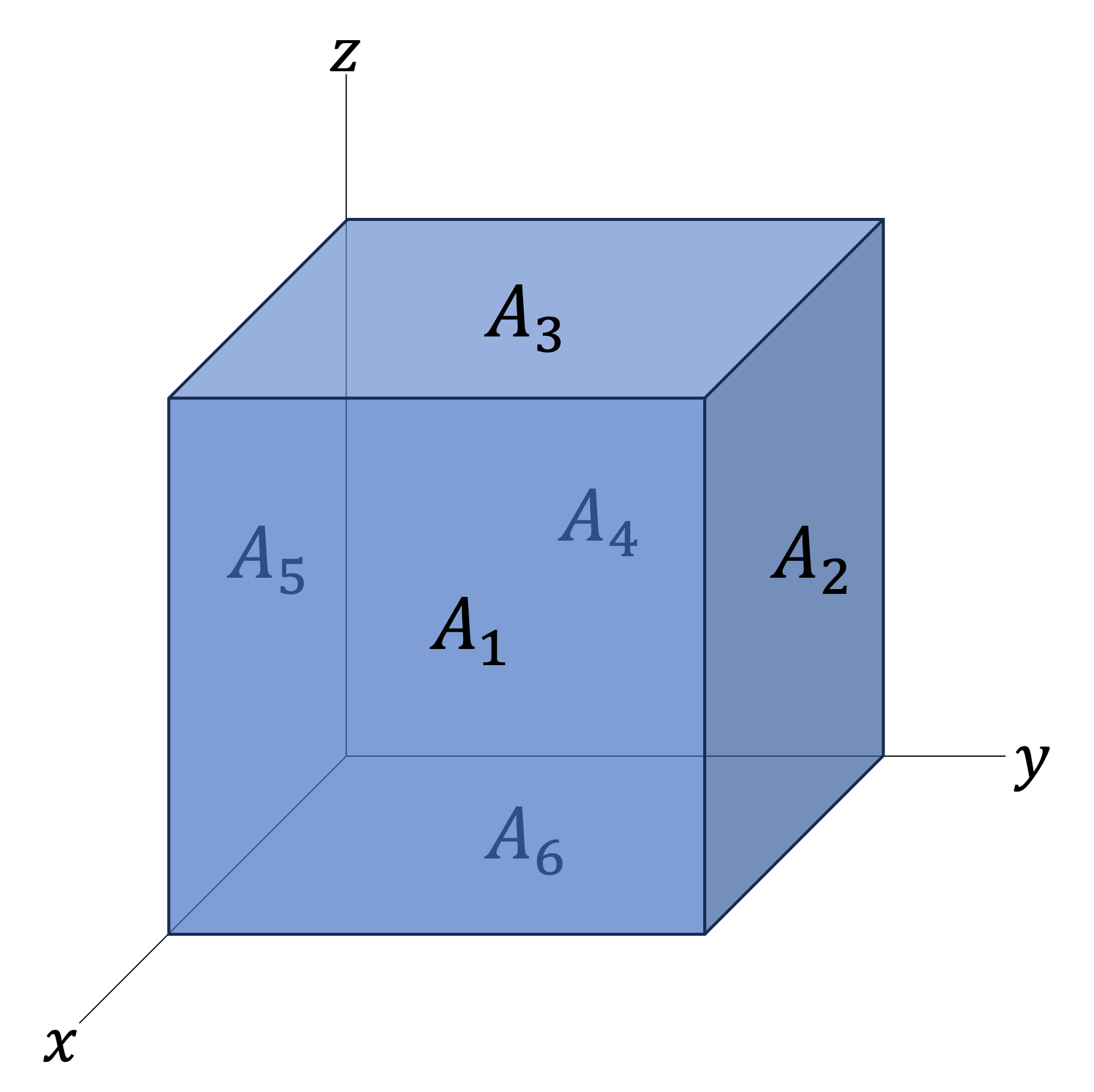
The six surfaces of a cube with length $~l_1~ m$ on each side, with $\vec A_1$, $\vec A_2$, $\vec A_3$ in the front, $\vec A_4$, $\vec A_5$, $\vec A_6$ in the back.
A cube measuring $~l_1~ m$ on each side is immersed in an uniform electric field with magnitude $~e_field_1~ V/m$, pointing at $~angle_with_axis_1_degree~ ^\circ$ [[return (~int_cw_or_ccw_1~ >0)? "counterclockwise" : "clockwise"]] to the [[return direction_axis_1]] on the $xy$-plane.
Write down his E field in vector notation.
Find the electric flux through each of the surfaces.
Draw a diagram of the electric field vector on the $xy$-plane and decompose using $\sin$ and $\cos$.
The area vectors of the six sides of the cube can be written down easily as $\pm A \hat i$, $\pm A \hat j$, $\pm A \hat k$.
Taking the dot product $\Phi = \vec E \cdot \vec A$ gives the flux.
Solution
The electric field vector on the $xy$-plane. There is no $z$-component because the question stated the field is only on the $xy$-plane.
E field
The figure shows the E field on the $xy$-plane. Decomposing the vector gives:
$$
\vec E = ([[return e_field_vector.string_mathjax(4, false)]] + 0 \hat k)V/m
$$
Area vectors
$\vec A_1 = + A \hat i = +(~l_1~ m)^2 \hat i = +[[return area_1 ]] \hat i m^2$.
Similarly, we have:
$$
\begin{eqnarray}
\vec A_2 &=& +[[return area_1 ]] \hat j m^2 \\
\vec A_3 &=& +[[return area_1 ]] \hat k m^2 \\
\vec A_4 &=& -[[return area_1 ]] \hat i m^2 \\
\vec A_5 &=& -[[return area_1 ]] \hat j m^2 \\
\vec A_6 &=& -[[return area_1 ]] \hat k m^2
\end{eqnarray}
$$
Electric flux
$$
\begin{eqnarray}
\Phi_1 &=& (+[[return area_1 ]] \hat i m^2)\cdot ([[return e_field_vector.string_mathjax(4, false)]] + 0 \hat k)V/m \\
&=& [[return sf_latex(+1 * area_1 * e_field_vector.x)]] Vm
\end{eqnarray}
$$
Similarly, we have:
$$
\begin{eqnarray}
\Phi_2 &=& [[return sf_latex(+1 * area_1 * e_field_vector.y)]] Vm \\
\Phi_3 &=& 0 Vm \\
\Phi_4 &=& [[return sf_latex(-1 * area_1 * e_field_vector.x)]] Vm \\
\Phi_5 &=& [[return sf_latex(-1 * area_1 * e_field_vector.y)]] Vm \\
\Phi_6 &=& 0 Vm
\end{eqnarray}
$$
The total flux is:
$$
\Phi_{total} = \Phi_1 + \Phi_2 + \Phi_3 + \Phi_4 + \Phi_5 + \Phi_6 = 0Vm
$$
This is the expected answer because the E field being uniform implies that there are no charges enclosed by the cube, which by Gauss' Law means the total electrix flux must be zero.