Currents can produce magnetic fields. This was the first hint to physicists that electricity and magnetism are secretly related. We focus first on the simple case of a straight long wire, which produces a magnetic field whose magnitude is given by:
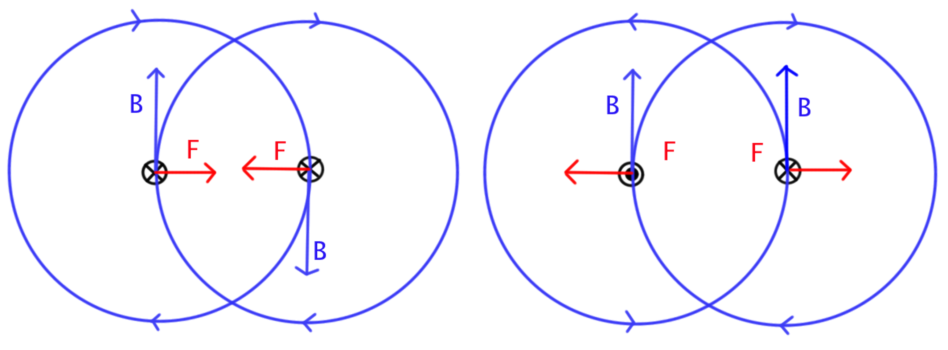
Since a current produces magnetic field, and any current interacts with a field via $\vec F = I \vec L \times B$, it means two currents placed side by side will interact through the magnetic fields they produce.
We focus on the case of two parallel wires carrying currents $I_1$ and $I_2$ (assume they have the same length $L$ for simplicity):
$I_1$ makes a field via $B_1 = \frac{\mu_0 I_1}{2 \pi r}$.
$B_1$ applies a force on $I_2$ via $\vec F_{21} = I_2 \vec L \times \vec B_1$.
$I_2$ makes a field via $B_2 = \frac{\mu_0 I_2}{2 \pi r}$.
$B_2$ applies a force on $I_1$ via $\vec F_{12} = I_1 \vec L \times \vec B_2$.
It turns out $|\vec F_{21}| = |\vec F_{12}|$, consistent with Newtons's third law of motion (action = reaction, but in opposite direction).
Simulation - Magnetic Field of a Pair of Currents (3D)
Magnetic Field of a Pair of Currents
Content will be loaded by load_content.js
Examples of what to draw in the exam.
Magnetic Field of a Coil
A loop of current is a magnetic dipole, producing a magnetic field similar to the electric field made by an electric dipole.
The Biot-Savart law gives the magnetic field $d\vec B$ produced by a small wire segement $d \vec l$ carrying current $I$.
$$
d\vec B = \frac{\mu_0}{4\pi} \frac{I d\vec l \times \hat r}{r^2}
$$
$d\vec l$ is the line segment pointing in the direction of the current.
$r$ is the separation between the segment and the observer.
$\hat r$ is the unit vector (i.e. $|\hat r| = 1$) pointing from the segment to the observer.
For a long wire (does not have to be straight), the total magnetic field is found by integrating over the whole wire:
$$
\vec B = \int \frac{\mu_0}{4\pi} \frac{I d\vec l \times \hat r}{r^2}
$$
Some books write the Biot-Savart law as (notice the $\hat r$ is missing):
$$
\vec B = \int \frac{\mu_0}{4\pi} \frac{I d\vec l \times \vec r}{r^3}
$$
It is equivalent to ours because $\hat r = \frac{\vec r}{r}$. However, this equation is not recommended because it hides the intrinsic $\frac{1}{r^2}$ dependence and diplays the misleading $\frac{1}{r^3}$ term instead. We should always try to write our equations in ways that makes the correct physics the most apparent.
Long straight wire
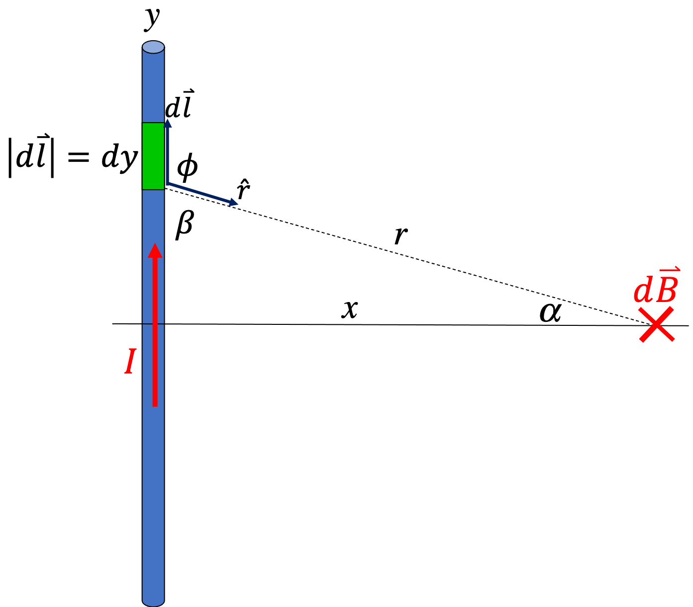
Using the Biot-Savart law to find the magnetic field at distance $x$.
We now apply the Biot-Savart law to an infinitely long straight wire to find the magnetic field at distance $x$. We are going to simplify our work by looking at only the magnitude:
$$
\begin{eqnarray}
B = |\vec B| &=& |\int d\vec B|
\end{eqnarray}
$$
In general, $|\int d\vec B| \neq \int |d\vec B|$, just like $|\vec u + \vec v| \neq |\vec u| + |\vec v|$ (try $\vec u = 2\hat i$ and $\vec v = -2\hat i$). There is one exception, which is when $\vec u$ and $\vec v$ are parallel. In our Biot-Savart integral, you can check that $d\vec B \propto d\vec l \times \hat r$ all point in the same direction (into the screen) for every segment of the wire. Because of this, we can safely assert:
$$
\begin{eqnarray}
B &=& \int |d\vec B| \\
&=& \int \frac{\mu_0}{4\pi} \frac{I |d\vec l \times \hat r|}{r^2}
\end{eqnarray}
$$
Looking inside the integrand:
$$
\begin{eqnarray}
|d\vec l \times \hat r| &=& |d\vec l| |\hat r| \sin \phi \\
&=& \sin \phi dy & \text{ because $|\hat r|=1$} \\
&=& \sin (180^\circ - \beta) dy & \text{ because $\phi=180^\circ - \beta$}\\
&=& \sin \beta dy & \text{ trig identity}\\
&=& \sin (90^\circ - \alpha) dy & \text{ because $\beta = 90^\circ - \alpha$}\\
&=& \cos \alpha dy & \text{ trig identity}
\end{eqnarray}
$$
We can also write $r$ and $dy$ in terms of $\alpha$:
$$
\begin{eqnarray}
\cos \alpha &=& \frac{x}{r} \\
\Rightarrow r &=& \frac{x}{\cos \alpha} \\
&=& x \sec \alpha
\end{eqnarray}
$$
$$
\begin{eqnarray}
y &=& x \tan \alpha \\
\Rightarrow dy &=& x \frac{d \tan \alpha}{d\alpha} d\alpha \\
&=& x \sec^2 \alpha d\alpha \\
\Rightarrow |d\vec l \times \hat r| &=& \cos \alpha dy \\
&=& \cos \alpha (x \sec^2 \alpha d\alpha) \\
&=& x \sec \alpha d\alpha
\end{eqnarray}
$$
Ampere's law is used to relate the magnetic field around a loop to the current enclosed by the loop:
$$
\oint \vec B \cdot d\vec s = \mu_0 I_{enclosed}
$$
Integral taken over a one-dimensional loop.
$I_{enclosed}$ is the total amount of current inside the loop.
The integration can computed in either directions (clockwise or counterclockwise).
Similar to the idea of Gauss' law $\oint \vec E \cdot d\vec A = \frac{q_{enclosed}}{\epsilon_0}$ (although Gauss' law intergrates over a two-dimensional surface).
The sign of the current is determined by the right hand grip rule:
Wrap your four fingers in the direction of the path integration.
Your thumb determins the positive direction for $I$.
Currents flowing opposite to your thumb are considered negative.
Content will be loaded by load_content.js
Straight wire
Ampere's law applied to a single current $I$, with a circular Amperian loop of radius $r$.
Applying Ampere's law to a single current, in the counterclockwise loop shown in the figure, we have:
$$
\begin{eqnarray}
\oint \vec B \cdot d\vec s &=& \mu_0 I_{enclosed} = \mu_0 I & \text{ because $I_{enclosed} = +I$ by right hand rule} \\
\Rightarrow \mu_0 I &=& \oint B \cos 0^\circ ds & \text{ because $\vec B \parallel d\vec s$} \\
&=& \oint B ds \\
&=& B \oint ds & \text{ because $B=constant$ by symmetry}\\
&=& B (2\pi r) \\
\Rightarrow B &=& \frac{\mu_0 I}{2\pi r}
\end{eqnarray}
$$
This is the magnetic field of a straight long wire that we used before.
Amperian loop in the cross-section of a toroid. The crosses and dots indicates currents flowing into and out of the screen, respectively. Only the currents flowing out of the screen are enclosed by the loop and contribute to $I_{enclosed}$.
Suppose a toroid has a total of $N$ turns. The total current enclosed by the Amperian loop as shown in the figure is $I_{enclosed} = NI$.
$$
\begin{eqnarray}
\oint \vec B \cdot d\vec s &=& \mu_0 I_{enclosed} = \mu_0 NI \\
\Rightarrow \mu_0 N I &=& \oint B \cos 0^\circ ds & \text{ because $\vec B \parallel d\vec s$} \\
&=& \oint B ds \\
&=& B \oint ds & \text{ because $B=constant$ by symmetry}\\
&=& B (2\pi r) \\
\Rightarrow B &=& \frac{\mu_0 N I}{2\pi r}
\end{eqnarray}
$$
Solenoid
Amperian loop in the cross-section of a solenoid, the top edge of the loop can be pushed to infinity where $B\approx 0$. Only the bottom segment of the loop contribute.
Suppose a solenoid has $n$ turns per unit length (i.e. turns density is $n$). Choose a rectangular Amperian loop as shown in the figure, and push the top edge to infinity where $B\approx 0$. This means the top edge does not contribute to $\oint \vec B \cdot d\vec s$. The right and left edge also do not contribute because $\vec B \perp d\vec s$ so $ \vec B \cdot d\vec s = 0$. Only the bottom edge is left in the integral.
$$
\begin{eqnarray}
\oint \vec B \cdot d\vec s &=& \mu_0 I_{enclosed} = \mu_0 I n w & \text{ because number of wires inside loop is $nw$} \\
\Rightarrow \mu_0 I n w &=& \int_{bottom} \vec B \cdot d\vec s + \int_{right} \vec B \cdot d\vec s + \int_{top} \vec B \cdot d\vec s + \int_{left} \vec B \cdot d\vec s \\
&=& \int_{bottom} \vec B \cdot d\vec s + 0 + 0 + 0 \\
&=& \int_{bottom} B \cos 0^\circ ds & \text{ because $\vec B \parallel d\vec s$} \\
&=& \int_{bottom} B ds \\
&=& B \int_{bottom} ds & \text{ because $B=constant$ by symmetry}\\
&=& B w \\
\Rightarrow B &=& \mu_0 n I
\end{eqnarray}
$$
This is the same equation that was given before for solenoid.


.svg)


_20_degree_split_ring.gif)