The general solution of the oscillation equation $\ddot{x} = - \omega^2 x$ is:
$$
x = A \cos(\omega t + \phi)
$$
$A$ and $\phi$ are found by the initial conditions. For example, an oscillator started from rest will have $\phi=0$ and $A= x_{initial}$.
| Name |
Symbol |
Unit |
Meaning |
| Amplitude |
\(A\) |
\(m\), or other units |
maximum displacement, or other meanings (such as angle) depending on the system |
| Phase constant |
\(\phi\) |
\(rad\) |
shift of the $\cos$ function along the $t$ axis |
Equivalent forms of the solution
Simulation - Graph of Simple Harmonic Oscillation
Graph of Simple Harmonic Oscillation
General solution to $\ddot{y} = - \omega^2 y$:
Calculations will appear here.
Math Review - Differentiation of Trignometric Functions
You need to know how to differentiate $\cos$ and $\sin$ functions to proceed further. We will start with two basic facts:
$$
\begin{eqnarray}
\frac{d}{d\theta}\sin\theta &=& \cos \theta \\
\frac{d}{d\theta}\cos\theta &=& -\sin \theta
\end{eqnarray}
$$
In physics we often differentiate with respect to $t$, like so:
$$
\begin{eqnarray}
\frac{d}{dt}\sin\omega t &=& \omega \cos \omega t \\
\frac{d}{dt}\cos\omega t &=& -\omega \sin \omega t
\end{eqnarray}
$$
Note that every time derivative "pulls down" a factor of $\omega$ due to the chain rule of calculus.
The last step is to include the phase constant $\phi$. Fortunately, $\phi$ just comes along for the ride and do not change the results:
$$
\begin{eqnarray}
\frac{d}{dt}\sin(\omega t + \phi) &=& \omega \cos (\omega t + \phi) \\
\frac{d}{dt}\cos(\omega t + \phi) &=& -\omega \sin (\omega t + \phi)
\end{eqnarray}
$$
Note that every time derivative "pulls down" a factor of $\omega$ due to the chain rule of calculus.
Differentiating $x = A \cos(\omega t + \phi)$, we get the velocity and the acceleration:
$$
\begin{eqnarray}
v &=& \dot{x} = A \frac{d}{dt} \cos(\omega t + \phi)= -A \omega \sin(\omega t + \phi) \\
a &=& \dot{v} = -A \omega \frac{d}{dt} \sin(\omega t + \phi) = -A \omega^2 \cos(\omega t + \phi)
\end{eqnarray}
$$
Another way to get to $a$ quickly is to use the simple harmonic equation $\ddot{x} = -\omega^2 x$:
$$
\begin{eqnarray}
a &=& \dot{v} = \ddot{x} \\
&=& -\omega^2 x \\
&=& -\omega^2 A \cos(\omega t + \phi)
\end{eqnarray}
$$
Because both $\sin$ and $\cos$ functions are bounded within $-1$ and $+1$, the general rule for finding the maximum value of such functions are given by:
$$
\begin{eqnarray}
\big( M \cos \theta \big)_{max} &=& |M| \\
\big( M \sin \theta \big)_{max} &=& |M|
\end{eqnarray}
$$
Applied to $x, v, a$ gives:
$$
\begin{eqnarray}
x_{max} &=& |A| \\
v_{max} &=& | A \omega | = |A| \omega \\
a_{max} &=& |A \omega^2| = |A| \omega^2
\end{eqnarray}
$$
Content will be loaded by load_content.js
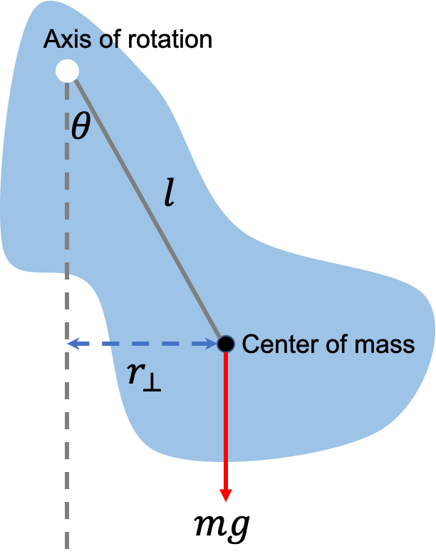
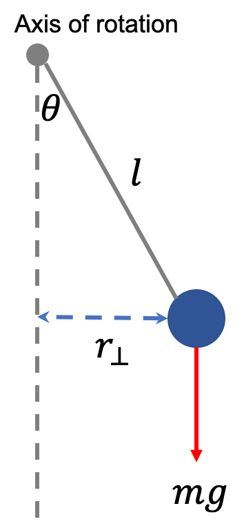
Angular variables
For angular displacement $\theta$ in $\ddot{\theta} = -\omega^2 \theta$ (such as a simple pendulum of length $l$), we have:
$$
\theta = \Theta \cos(\omega t + \phi)
$$
where $\Theta$ is the amplitude of the angular motion (plays the role of $A$).
The angular velocity and acceleration can be found by differentiation just like before:
$$
\begin{eqnarray}
\dot{\theta} &=& \Theta \frac{d}{dt} \cos(\omega t + \phi)= -\Theta \omega \sin(\omega t + \phi) \\
\ddot{\theta} &=& -\Theta \omega \frac{d}{dt} \sin(\omega t + \phi) = -\Theta \omega^2 \cos(\omega t + \phi)
\end{eqnarray}
$$
We did not use the usual notation $\omega$ for angular velocity because we already used $\omega$ to represent the angular frequency of the oscillation. Instead we simply write the angular velocity as $\dot{\theta}$, the angular acceleration as $\ddot{\theta}$ to avoid confusion.
Using $s = l \theta$ (definition of radians), we can find the tangential speed of the pendulum of length $l$ by:
$$
\begin{eqnarray}
v &=& \dot{s} = l \dot{\theta} \\
&=& -l \Theta \omega \sin(\omega t + \phi)
\end{eqnarray}
$$
_152.jpg)